Artificial Intelligence is for making good predictions (mostly), and Bayes is the OG (original gangster) prediction formula. Bayes was perhaps the first stab at creating an artificial intelligence algorithm. While it has limitations, it continues to be a great starting point for learning how to think probabilistically, which is the essence of machine learning. For those who struggle to memorize Bayesian formulas, I will us this post to show how a lesser known expression of Bayes Rule can lead to better retention and understanding, as well as computational empowerment.

Specifically, I hope to demonstrate how the Odds Vector Form (hereinafter also referred to as the OVF) gives us much better Bayes formulas than the most commonly used Probability Form. The visual elegance of the improved formulas commits itself much more indelibly to memory. Additionally, the OVF allows us to deploy Bayes in many more dimensions, easily... like by hand, even. The Odds Vector Form gives us a totally memorable formula for Bayesian inference with multiple initial hypotheses, (rather than the classic case of a simple binary), and with hundreds (or even thousands) of conditionals.

In short, the "Odds Vector Form" makes it much easier to see which basic components operate in conditional probability, and what exactly is happening to those components, when we calculate posterior probabilities. Once we get a handle on the core components and basic operations, it's much, much easier to (1) remember Bayes forever, and (2) think in additional data dimensions.

Why is it desirable to think in additional data dimensions? Because people (and machines) reach conclusions using multiple pieces of evidence, not just one. It's totally legit and even darling to start any mathematical inquiry in limited dimensions, and build up from there. But in real life, learning always involves way more than one piece of evidence. Our Creator (or Randomness, depending on your lexicon) made us extremely perceptive and sophisticated machines, and every intuition, decision, or judgment we make, involves hundreds or thousands of pieces of evidence.

Ultimately the OVF is about organizing yourself for success. Mary Kondo would be so proud. I hope that by the end of this post, you too will have gained an unshakeable understanding of Bayesian Inference. Without further ado, let's delve!

Odds vs. Probability?

Before I can adequately explain the difference between the OVF and the probability form of Bayes, I should very briefly explain the difference between odds and probability in general. The OVF is not different in substance from the probability formula. Rather, it is simply a different expression of ratios, as if it were the same concept in a different language. Thus, knowing how to convert probability to odds in general, (like knowing how to translate from French to German), will be key in grasping the new expression.

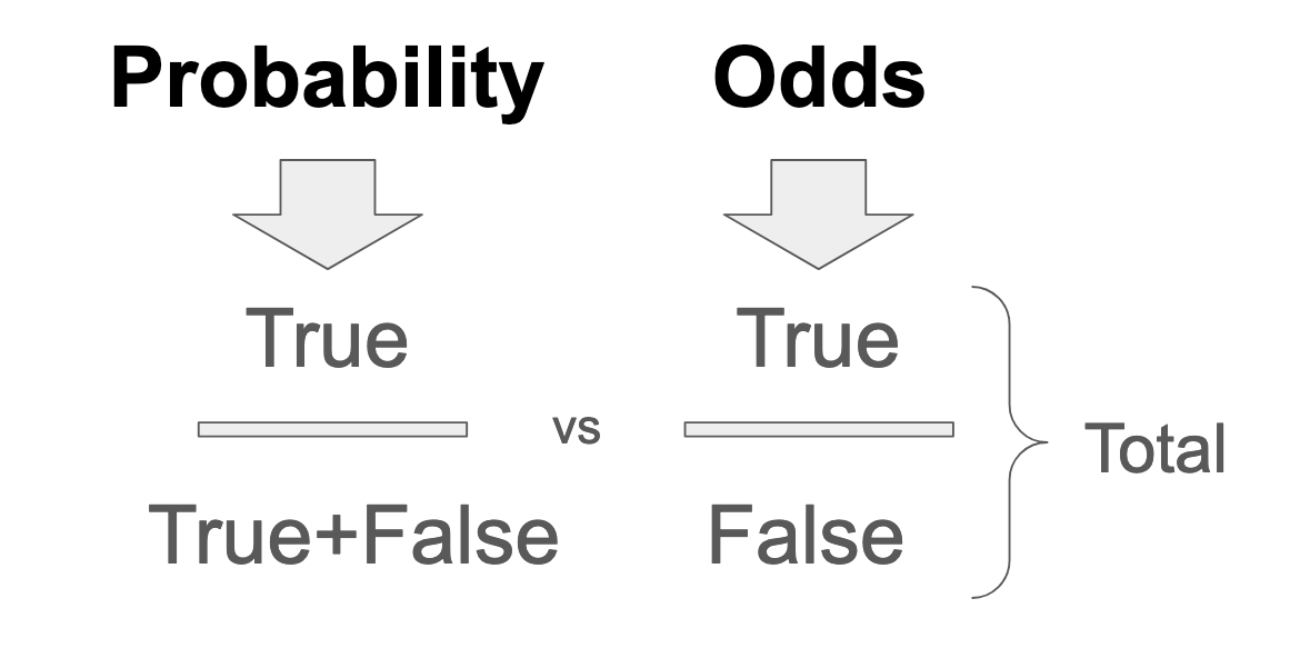
Probability as a mathematics discipline is about ratios of inclusion in a set of possible outcomes. There are at least three different ways I can think of to express a ratio: (1) Fractions, (2) Percents, and (3) Odds. Probability is expressed as a fraction of a total, benchmarked to 100. Odds, on the other hand, are expressed in relative frequencies. A fifty percent probability is the same as one-to-one odds:

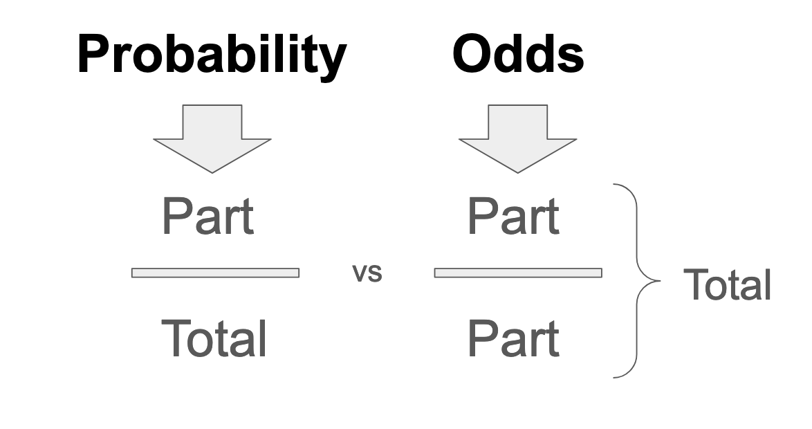
In other words, if inclusion in any given probability space is represented as an odds ratio, the probability expression of that inclusion, by definition, contains the "numerator" of the odds ratio fraction, duplicated in the denominator. In the case of binary boolean outcomes, for example, probability is expressed as True/(True+False). Whereas, odds for the same binary are expressed as True/False. In the case of nonbinary outcomes, the denominator of a probability contains the total probability space, which is the set of all possible outcomes. Odds have no denominator, and the way to create one it to add up all parts.

This definitional fact about the structure of probability vs. odds will come in handy as we move forward. The conversion from odds to probability is sort of self-explanatory, but clearly it involves subtracting the numerator from the denominator for probability-to-odds, or totalizing the denominator, for odds-to-probability. Now that we have grasped the difference between odds and probability ratios, let's move forward with rewriting the classic Bayes form!

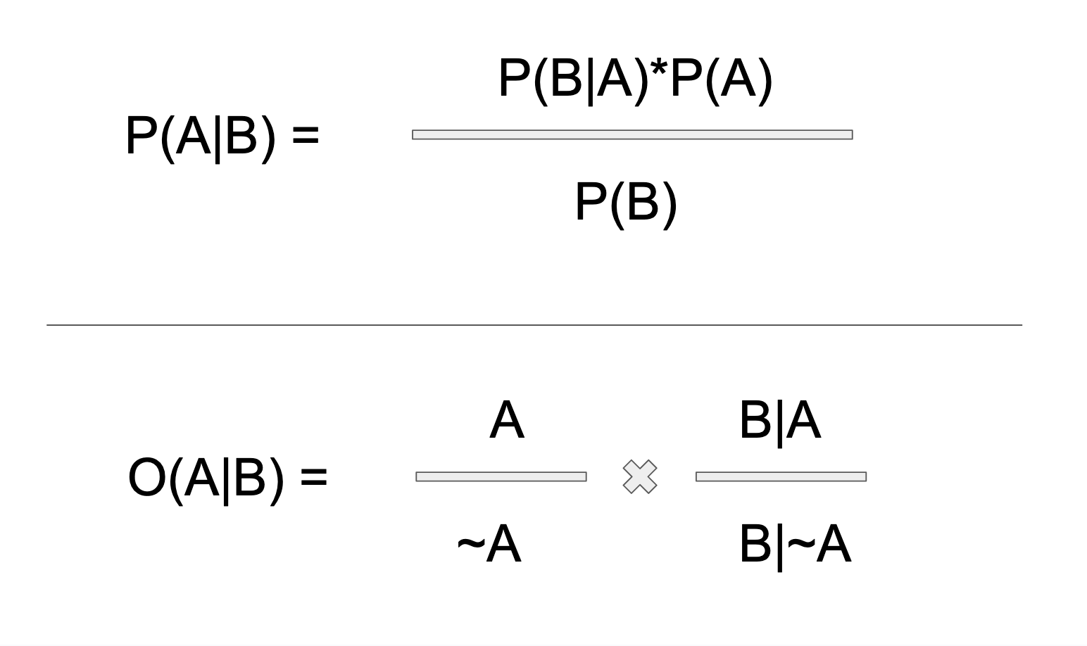
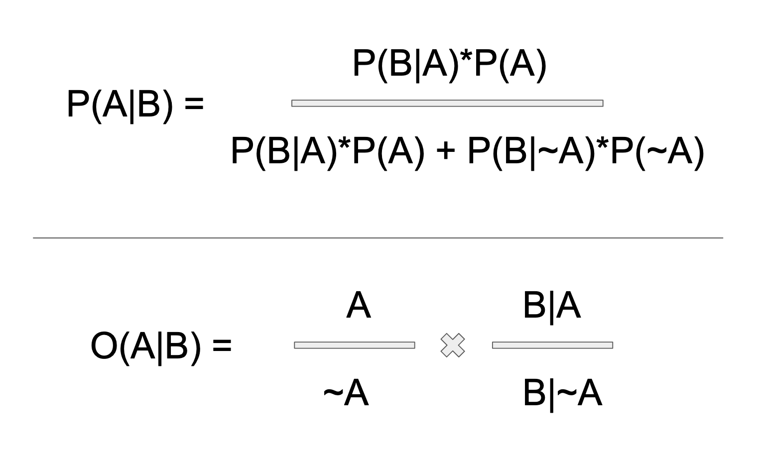
Below is Bayes Rule written two ways. On top is the classic probability form, versus on the bottom, which is the odds form. Maybe the probability version doesn't look so bad at first glance. But the denominator is deceptive. The denominator is the marginal probability of B, i.e. the probability of B happening at all. Because B is conditioned first by A, (on the right hand side of the equation, which is the side where we are conducting our computations), P(B) resolves into all of subordinated possibilities of A. In a binary split of A, this includes (B|A) and (B|~A). In other words, B|A gets weighted by the probability of each of the possible universes of A-ness, in which it resides.

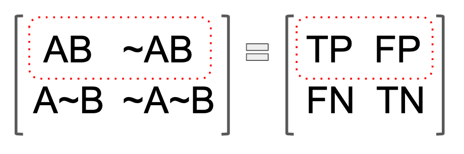
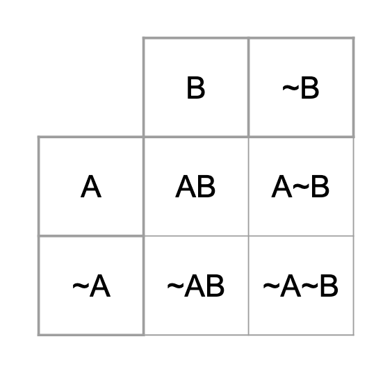
The rather sloppy point I am trying to make about the denominator in the above graphic is much easier to grasp in the language of true positives and false positives, which is why it's a pedagogical favorite to use diagnostic testing. In other words, B happens both when A and ~A happen. On the surface of the question, it may seem like not-A isn't a universe of A at all. And in a standalone A, not-being-A would in fact not be a universe. But in a conditional A, there are going to be occurrences of B co-occurring with ~A; these would be the false positives.

Here is the expanded version of the denominator. As you can see, it looks quite a bit harrier than the unexpanded version:

The expanded version is revealing, however. Squint your eyes at it, and a pattern may begin to emerge... The duplicated numerator in the denominator! Below I have encircled the duplicated numerator within the denominator of the probability version (in red). By conversion to odds, this redundancy in the denominator can be "factored out." Keep in mind, this isn't true algebraic factoring, as the redundant piece simply never factors into odds to begin with. If we translate the ratio, using an odds ratio expression instead, what emerges is a much cleaner fraction, whose denominator does not need to be summed for each hypothesis at every step.

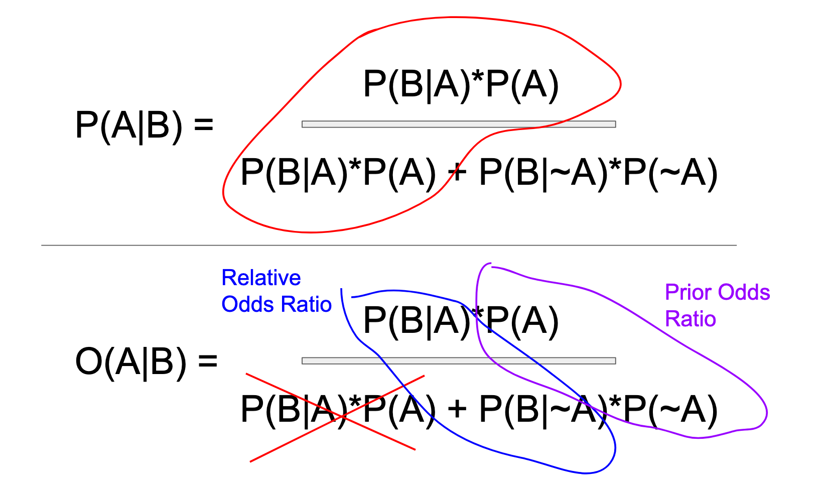
The other pattern that should begin to emerge is the simplicity of the remaining components. Basically, you have two ratios hidden in and hopelessly intermingled in the denominator, in the probability formula. The ratio of A to not-A. And the ratio of B-given-A, to B-given-not-A. That's it! That's all Bayes is. In two dimensions, in a hundred dimensions, in a million dimensions, the odds ratio becomes an odds vector, but does not fundamentally change in essence.

At this point, I think it is worth carrying out a number of worked examples. First we will run through an example in two dimensions. Then we will work through an example with three dimensions. Finally, we will close with some caveats.

Example I: Two Dimensions

In another blog post, we created a solutions matrix, which maps out the probability space, created by the intersection of the two binary vectors A and B. In order for the vectors to come out right within the conventions of matrix multiplication, I organized my hypothesis matrix with the hypotheses on the diagonal, and the evidence array with each piece of evidence in its own column, (duplicated down the column as many times as necessary to equal n number of columns of the first matrix, to mimic a real dataset array).

The above matrix multiplication is not the only way to generate a solution space. Since I have been thinking in matrices for a few months now, this feels the most intuitive to me. It's just my own made-up convention to think through the idea of every component in an array interacting with every corresponding component in another array. If it feels more intuitive to you, use a table: A table is just a geometric convention, which shows the components of two vectors intersecting with each other. See below:

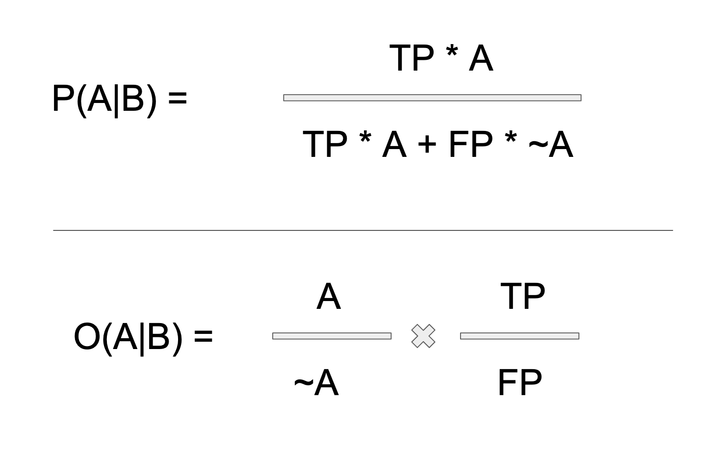
Let's take the classic diagnostic test example: Given that I tested positive for disease X, what are my chances of having the disease? In the classic example, we start with a positive test result, B. We want to know how likely it is that we have the disease. Thus, we only care about the B axis (versus the ~B axis) of our solution set, which in turn means that our formula is only going to include the TP (true positive) and the FP (false positive) terms. We don't care about negative test results, (though if we did, it would be the ~B axis, which we would focus on). I have encircled the axis of concern below:

The formulas we wish to solve, in terms of true and false positives is shown below:

I tidied all of the components needed to solve the above equations, in the table below. In order to perform some actual calculations, I bring in the empirical rates values from a problem I solved in another blog post. In that post, we assigned a 1% prevalence rate to the disease, and we posited a diagnostic test that was 95% accurate (both for sensing positives, and for specifying negatives). Remember that in real life, all of these rates would come from empirical research or estimation. These are not rates that can be theoretically derived! Also, in real life, there may be some difference in test accuracy as sensitivity vs. specificity. Let's just agree not to care about this for now.

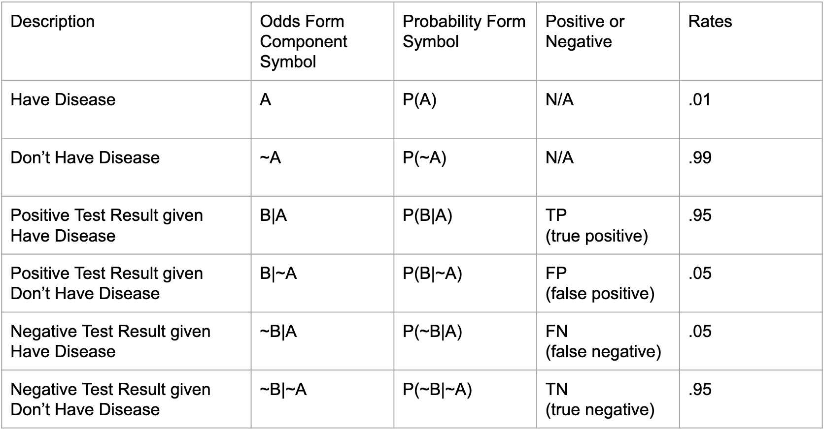
The first thing to notice in this table is that all of the conditional probability rates are in terms of A. That is, all of the probability rates are in terms of being sick or not sick. Though we start with a positive test result (B), in order to calculate what that means, all of our rates pertain to the likelihood of being sick, which is the flip side of the equation. I like to say that Bayes Rule is a mirror for flipping from one universe to its inverse (this is explained in great detail in another blog post). Thus, when we want to find (A|B), we solve for the mirror universe (B|A), and vice versa.

In other words, though our posterior is in terms of B, our priors are in terms of A, which will allow us to wormhole ourselves into the mirror world, so to speak. Let's plug in some numbers from our handy dandy Mary Kondo table of values! Again, to compare both forms of the formula. The probability form versus the odds form:

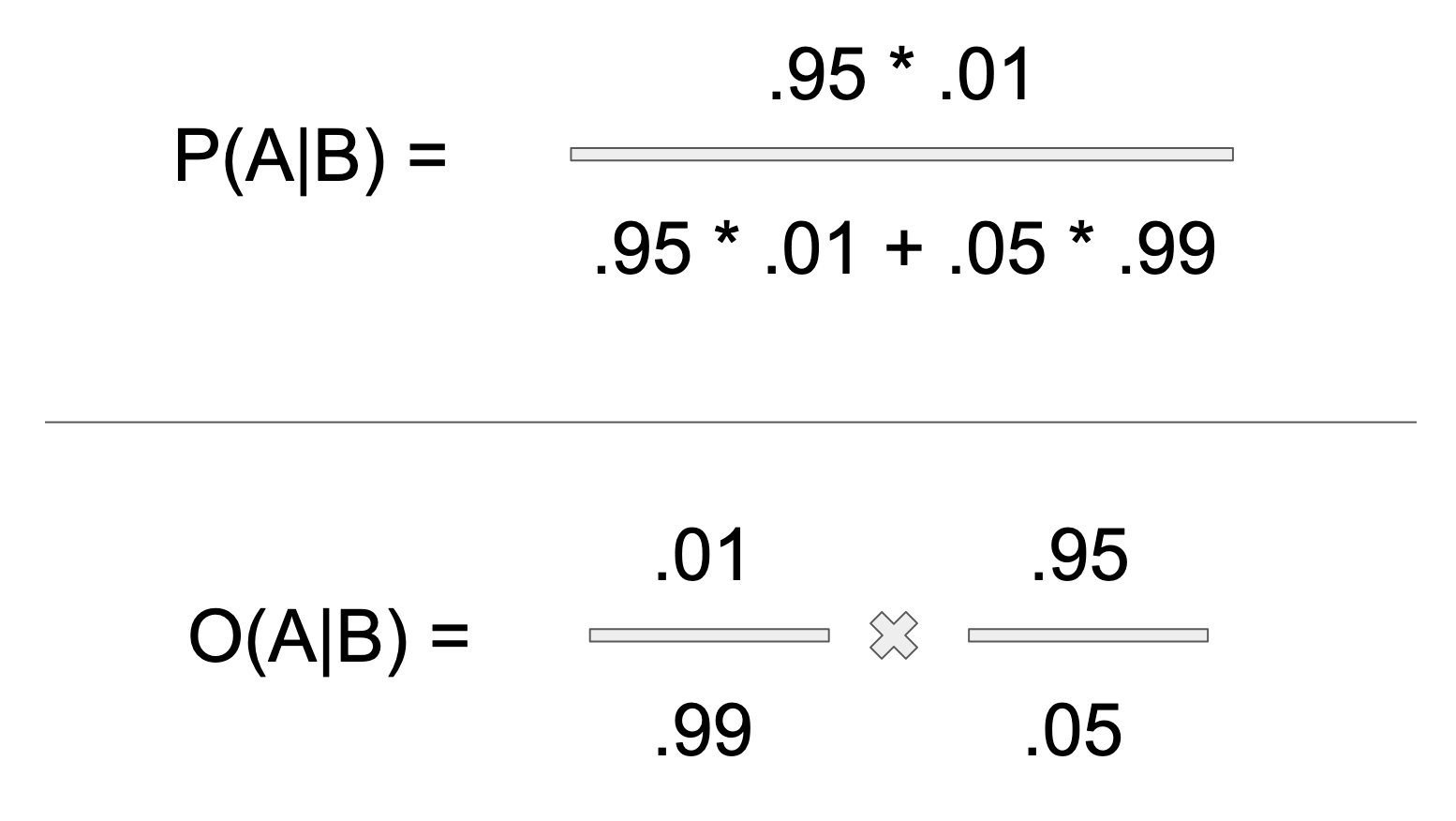
Again, remember that the odds form is not really different from the probability form. It's just a different expression of the same underlying ratio, like saying something in Spanish versus French. It works. It obviously works–not because anything was factored out of the denominator–it simply never factors into the denominator in the first place. After all, the method for converting odds to probabilities in general is to add the numerator to the denominator. Conversely, the method for converting probabilities to odds is to subtract the numerator from the denominator:

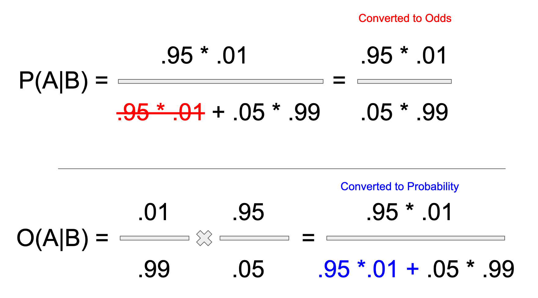
As a visual and verbal mathematician, I like when it's just plain obvious why something works, without the requirement for crunching any numbers. The important part is this: In the probability form of Bayes Rule, the priors, that is, the marginal probabilities of A and ~A, are hopelessly intermingled in a summation with the rates of B given A and ~A (the Bayes Factor). Whereas in the odds form, we get a much cleaner schema of components, with one ratio for priors, and another ratio for the update of those priors.

Often the "update" ratio of relative likelihoods is called the "Bayes Factor." That term does nothing for my intuition, personally, so I avoid it. But I feel it's worth noting, in case it is something that resonates with you... The best explanation I have heard for the Bayes Factor is the ratio of how much likelier it is, than not, to witness your piece of evidence given the hypothesis. This wording does feel intuitive to me, and it is how I think about learning, especially when faced with unpleasant and potentially traumatizing evidence. Like, for instance, the smell of wildfire smoke. But I digress...

Finally (and this is crucial), when using odds, you probably need to convert back to probability at the end, to effectively communicate your results. Don't ask me why 100% is the intuitive total for humans. Possibly because we have ten fingers and ten toes, and thus find it intuitive to count in sets of ten. Possibly God really likes decimals and cents. I can't say. The solution for this problem is going to be a percent chance of having a disease, though. That is a given. So in order to communicate our solution effectively, we will need to speak in terms of per-cents.

Diagnostic testing provides very intuitive terms like "false positive" and "true positive," but this example can be generalized to any set of binary vectors. The first step towards extrapolating from two data dimensions to three or more is to think in terms of vectors. Technically, a ratio is a vector with two dimensions, but I certainly don't think of it that way by default. Once a third number enters the arena, the tripartite ratio becomes pretty obviously a vector.  Ultimately Bayes has two main ratios, which can be thought of as two vectors. These two basic vectors do not change, no matter how many conditionals you add to Bayes.

Example II: Non-Binary

So far we have been dealing with a binary hypothesis example. If we were to draw the probability tree, which expresses this example, the first fork in the tree would be a bifurcation into two trunks, each with two branches. The diagnostic test, with its neat binary options of sick/not sick, positive/not positive, is a great starting point. But in real life applications, there are so many more possibilities than just those two. The classic non-binary classification problem is, of course, the spam filter. But we need not think merely in terms of spam filters. Classification has so many applications. Life would not work without determining what is what.

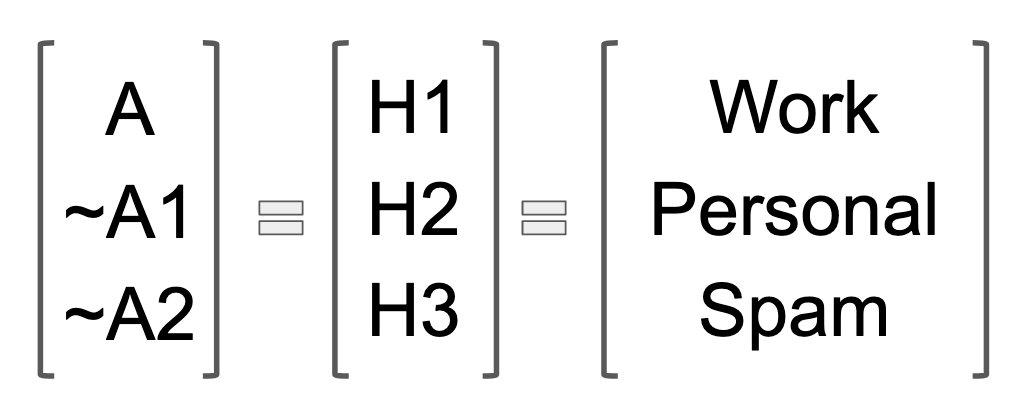
For me, the easiest way to transition from the notion of a ratio to that of a vector is by thinking of the original A/~A as still operative, except that there are multiple ~A's. In the spam example, there is the possibility that the email is spam, but there are multiple ways to be not-spam. A not-spam email could be business or personal (or a million other things probably). For the sake of our calculations, rather than have a bunch of A's, ~A1's and ~A2's gumming up the formulas, it's useful to switch to "H" (for hypothesis) notation.

Rather than reinvent the wheel, I am going to borrow a spam filter example from Arbital dotcom. Note: Even though I will be using the same values and labels from Arbital, they do not include the proof of (or any explanation of) the probability version of the formula. All of the visuals and the writing you find here are my own original work. Also, I have substituted the name of the category "Work" for Arbital's "Business" category, mostly because the word "work" is shorter.

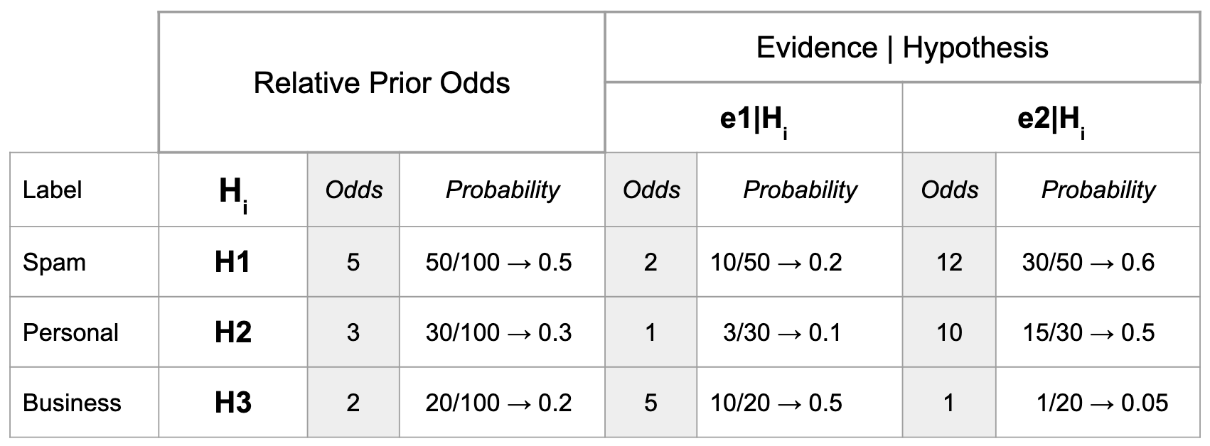
Background: Suppose that there are three categories of email: Work, Personal, and Spam. A user hand-labels the last 100 emails has labeled 50 as Work, 30 as Personal, and 20 as spam.  The word "buy" has appeared in 10 Work emails, 3 Personal emails, and 10 Spam emails.  The word "rationality" has appeared in 30 Work emails, 15 Personal emails, and 1 Spam email.

Problem to Solve: If an email contains the phrase "buy rationality," then what are the chances that it should be categorized as Work?

As before, I made this handy table, to organize all of the pieces of data that we do have. In order to make the comparison of OVF to probability easier to see, I've expressed vector components in both odds and probability.

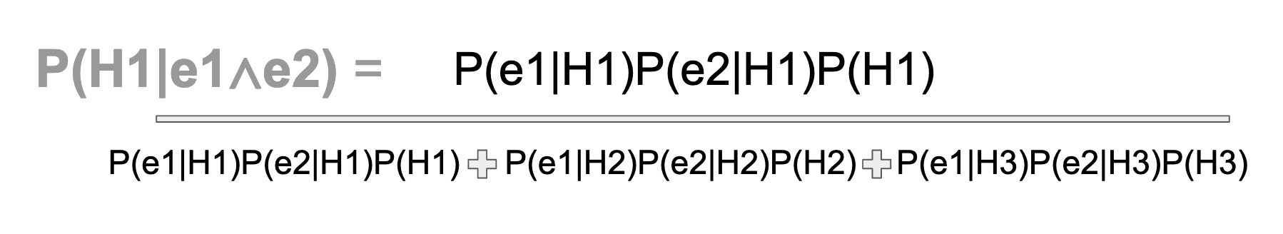
Let's see what the probability version of the formula would look like with two pieces of evidence. Here is the deceptively simple, unexpanded version of the formula. As before, the denominator is going to get really ugly, really fast:

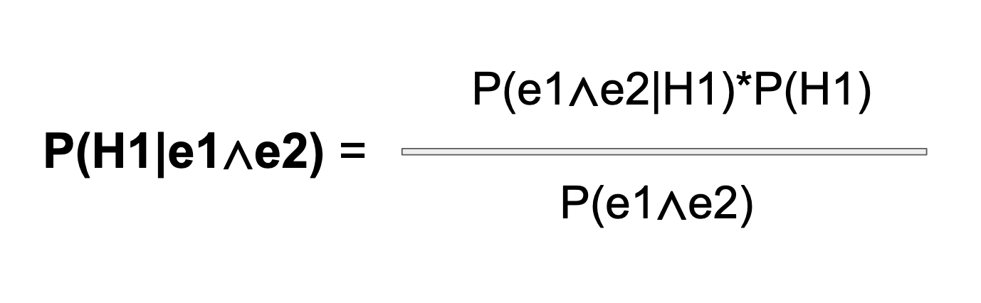
Right away, we have a big problem: Our formula contains terms, both in the numerator and the denominator, for which we lack any probability rate. We do not have a rate for the possibility of "buy" and "rationality" co-occurring in the same email, which means we do not have a probability to plug into the denominator term, P(e1∧e2). The same problem applies to a lesser extent to the (e1∧e2) term in the numerator. Recall that the the empirical research, upon which our word problem rests, identified when either "buy" or "rationality" appeared in the categorized emails.

In general, we don't know how many of the buy-word emails also contained the word rationality. And we certainly don't know the prevalence of the evidence words in each of our three hypotheses. Initially, it feels like we couldn't possibly figure out the word problem, in the absence of this knowledge. But there is a way to solve, and it involves making a fairly grand assumption. This assumption is that our various pieces of evidence have no bearing on each other. Neither piece of evidence materially impacts the likelihood of any other piece of evidence.

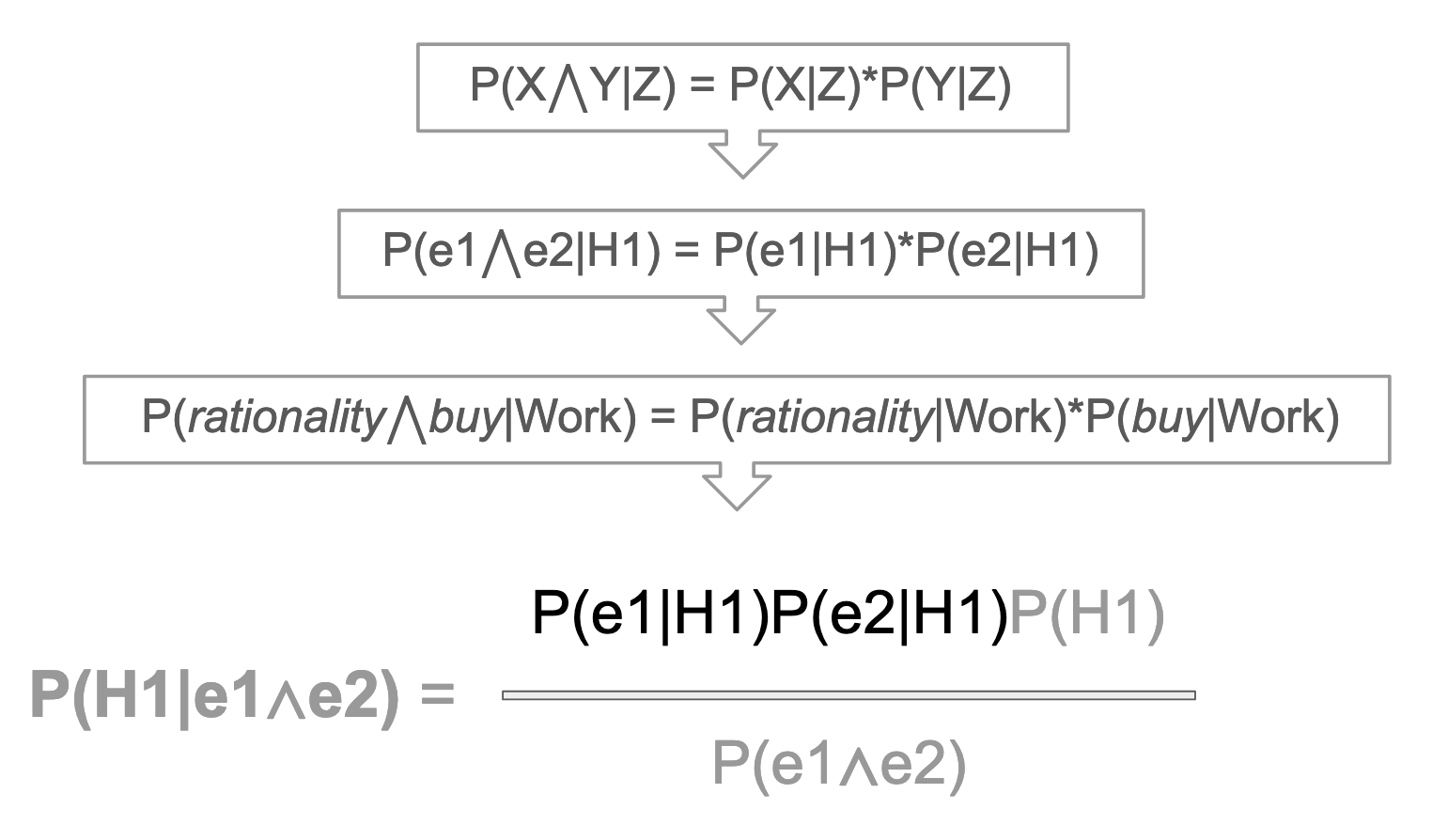
If we assume independence of the conditional terms, "buy" and "rationality," we can use the power of math to reorganize our formulas and make some substitutions, which render the (e1∧e2) term solvable. It's important to note that we are almost certainly incorrect in assuming independence of evidence. If an email contains the word "buy," that probably is a strong indicator for other words. It's true that models are not reality–that doesn't mean they don't give us useful information–and for now, we will just need to live with that.

So, assuming independence of evidences, we can fix the numerator first of all. Conditional probability is the same as regular probability, and the probability of two independent events happening together is a simple multiplication of the probability of each event happening separately. Like, the probability of flipping a coin heads two times in a row is just 1/2*1/2. Same goes for conditional probability, except the conditioning variable tags along.

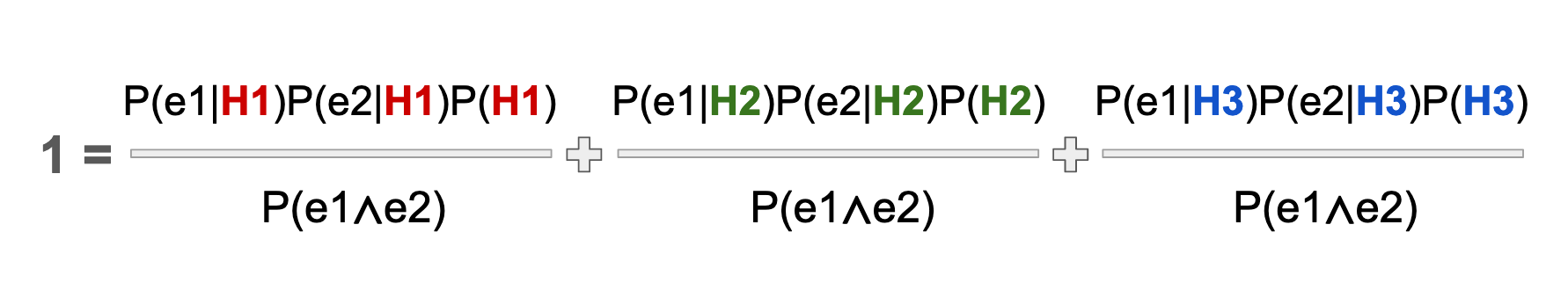
Now that we have fixed our numerator, we have to fix the denominator. The denominator is a little trickier, because, again, we don't have the data about how often the word "buy" co-occurs with the word "rationality" in any emails, much less within our three hypotheses. Nor do we have probabilities for how often those words appear in general. We will need to use the one piece of certainty that we do have, which is that the sum of all three conditional hypotheses equals 1. In other words, no matter what happens, we know that the message is one of the three: Work, Personal, or Spam, because these are comprehensive categories, by definition.

We just need to write out the formula above, three times: One for each hypothesis, and set their sum equal to 1. I have color coded the three respective hypotheses to make the pattern easier to see.

Now we can multiply all terms by the denominator to achieve the following expression. Voila! Now we have the denominator defined, like magic!

Finally, let's put the new, solvable denominator back into the original equation.

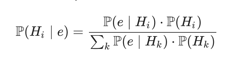
Whew! That was a lot. Below is (more or less) the generalized expression of the formula, which we just derived, although the evidence term needs i and k subscript notation to indicate that we have a vector of data, just like the H term. For multiple evidence conditionals, the numerator turns into the product of all data, given the hypothesis in question, weighted by the hypothesis in question (the prior). The denominator becomes the sum of the numerator term, summed over all possible values of the evidence, each time weighted by every possible hypothesis. Again, it's an ugly formula, and I don't like it. For a discrete probability, I would avoid it.

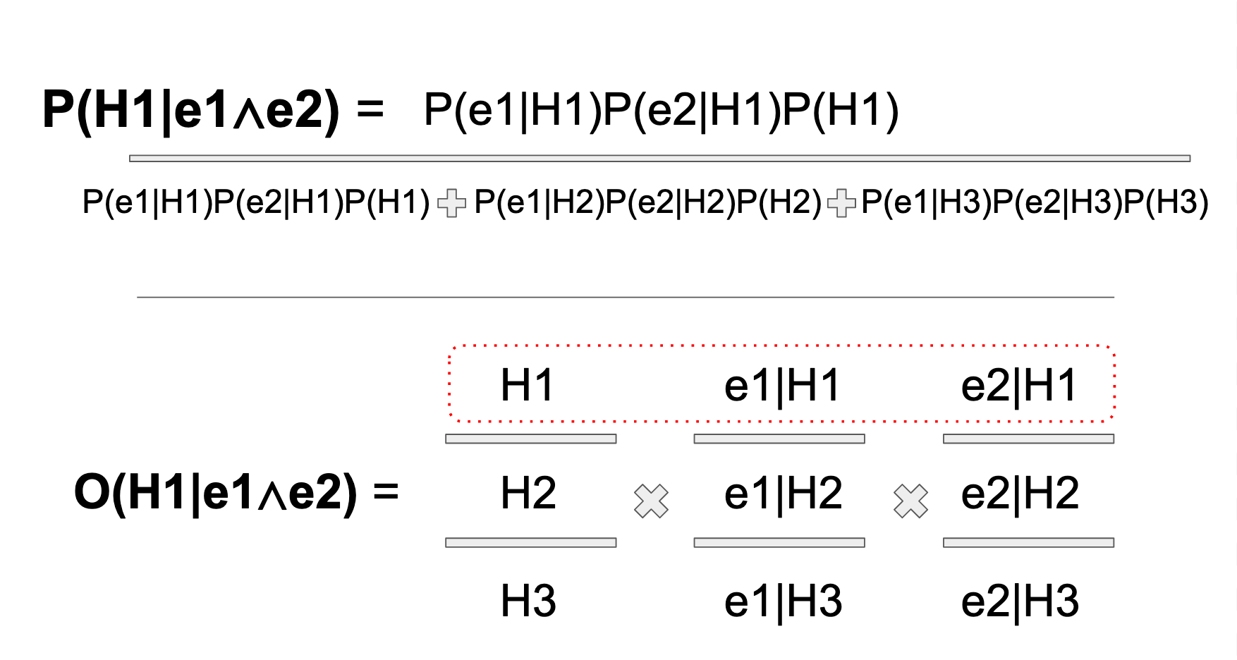
Here I hope the Reader can begin to truly appreciate the elegance of the odds form versus the probability form. I don't know if it's ADHD or what, but looking at this formula makes me feel crazy. I don't like it. I don't like it one bit. If I had to memorize it for a standardized test, I'd be S.O.L. Below shows the comparison to the Odds Vector Form, and there is almost no comparison. The visual presentation of the OVF, in my mind, is unforgettable. You've got your vector of priors, and then your relative odds, given those priors. Thing I know times thing I learned, given what I know, equals new thing I know.

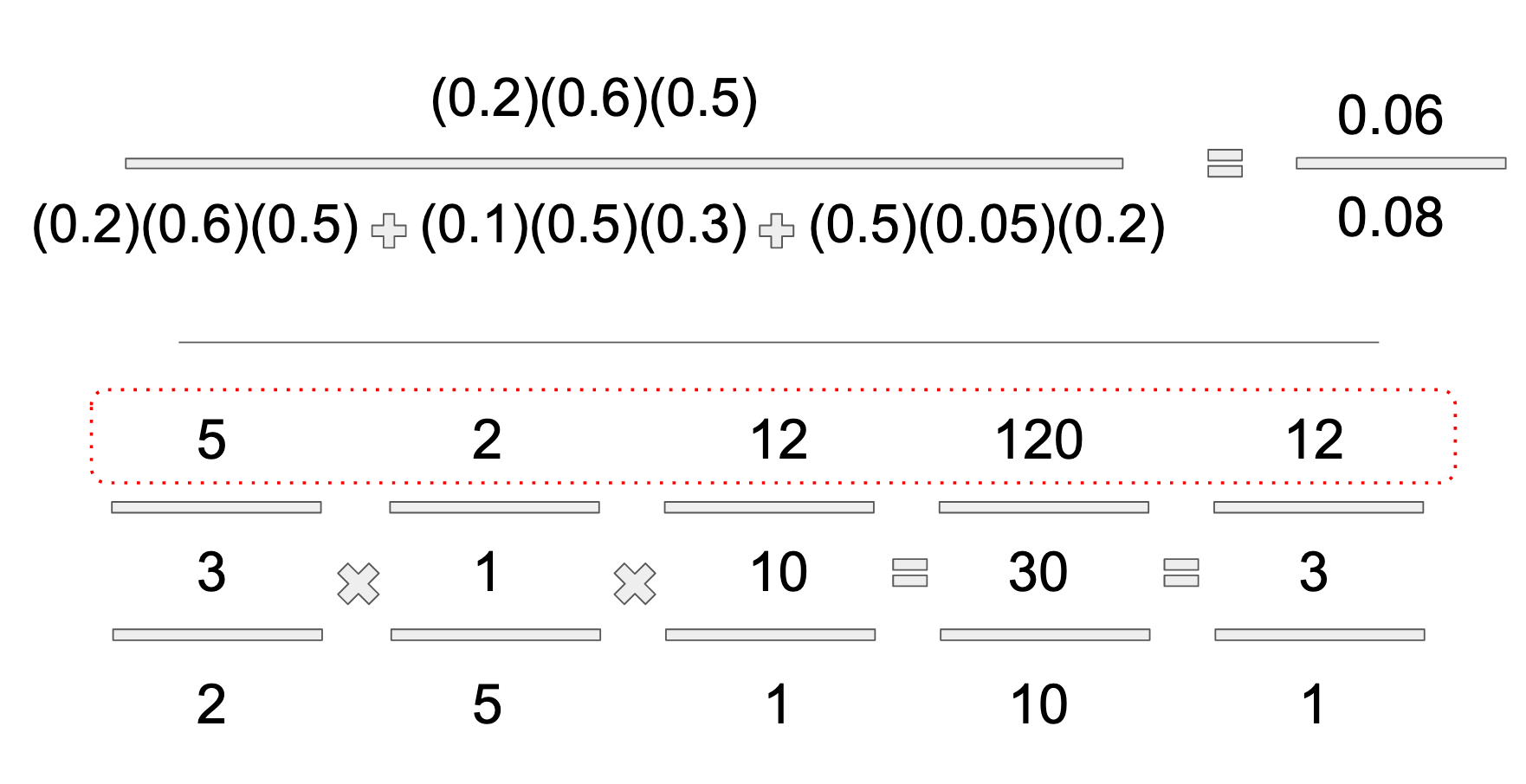
Now I just need to prove that it actually works. And it does! As Gil Strang would say in triumph, "the damn thing came out right!" The answer to the word problem is this: If we receive an email containing the phrase "buy rationality," there is a 75% chance that it's a "Work" email. Here are the fully worked out solutions for the above formulas.

Isn't it beautiful? It's better than a Hollywood nose job.

I know what you are thinking. Where the hell is 75% in the above solution diagram? In the probability formula, I hope it's easy enough to see that 0.06/0.08 reduces to 3/4ths, which easily converts to 75%. The odds ratio takes an extra step at the end of coming up with a totalized denominator, in order to convert each odds figure to a percentage. For ease of explanation, I went ahead and reduced 120:30:10 to 12:3:1. As already shown, to convert odds to probability, add up all of the numbers in your vector, and that makes your denominator. 12+3+1=16, which is the total and the denominator for that vector. No need to simplify the odds prior to probability conversion. 12/16ths is equal to 120/160ths after all!

Besides the visual elegance, and the ease with which the OVF commits itself to memory, the other major benefit is that the computations solve for all possible hypotheses simultaneously. We learn that the first hypothesis, H1, has a 12/16th or a 75% chance of being the case, given the evidence. But we can also readily see that H2 = 3/16ths and H3=1/16th. With the probability formula, additional computations would be required.

The other nice thing about the Odds Vector Form is that it empowers the user to solve complex conditional probability problems easily and by hand, or to program a script to do so. Rather than be totally reliant on out-of-the-box models from scripts, understanding the OVF empowers you to write your own. All you need is a vector of relative prior odds times your vector of relative evidence likelihoods (your "Bayes Factor" from the two tier example).  Instead of the prior odds being twofold, as they are in a fraction, they are column of relative odds.

Not sure how controversial a statement this is, but I don't think of odds form as being different from vector form. Because odds are not totalized, they can keep stacking, unlike probability. This works with multiple evidences too, or rather, multiple evidence vectors. Once you include more than two hypothesis vectors and more than one evidence vector, things begin to get more plow horse method. As below (thanks to

Staying Honest: A Few Caveats

This is the section where we come down off of the high of figuring out something cool, and reintroduce new doubts, one by one. No wild party or trip is complete without the comedown. So let's get on with it! As with any abstraction, there are a number of caveats to keep in mind. This by no means is a comprehensive list of potential things to consider.

The first caveat

...deals with discrete vs. continuous probability. In the examples we have worked out, the sought-after solution was the probability of a discrete hypothesis, given discrete pieces of evidence. However, it makes sense to wonder how we would assess the probability that our hypothesis falls within a range of values. Or our sample data may themselves consist of a range of continuous values, rather than discrete pieces of evidence. Or both. We could have a probability density function for a hypothesis, and multiple kinds of evidence.

In other words, in this blog post, we sought to answer the question, What is the probability that a discrete hypothesis is true, given discrete instances of evidence? But what if instead we wish to know, What is the probability that my hypothesis falls withing a range, given a range of evidence? The good news is this: The two basis ratios of Bayes–priors and likelihoods–remain the operative vectors in our problem. However, our formula will need some calculus. Remember the area under the curve (from calc class)? That's how you derive the probability of a range of continuous values, i.e. by taking the integral, which is the sum of all possible values within a range.

The continuous formula, for one hypothesis, and range of values for one piece of evidence, will look like this:

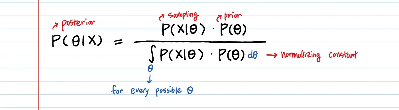
Again, the logic of the mirror world dictates that we will need to know the probability that evidence falls within a range, given a hypothesis, if we seek to know the probability of a hypothesis, given a range. The probability that evidence falls within a range is akin to a sampling distribution. The prior probability of a continuous hypothesis, on the other hand, would involve selection of a distribution that describes the evidence thereby implied.

We probably need a whole other blog post to explore the insertion of one or multiple integrals into our formulas. But for now, the word count on this post is getting grim. In the meantime, I refer the reader to Ms. Aerin's excellent Medium blog on Towards Data Science, for tips on how to use integrals.

The second caveat

...pertains to our assumption about the independence of evidence, which we already noted is almost certainly false, but we should dig into this a bit more. Again, the Naive Bayes assumption is that each class of evidence has no bearing or interaction with any other class of evidence. In our example, if the word "buy" were to have strong negative or positive correlations with the word "rationality," then an assumption of naivete may drastically over-count, or under-count, the resultant probability of the hypothesis, when these two words occur together.

There are lots of ways to deal with interactions between parameters in a model. For simple models, the solution could be to hard-code logic with good old if-else scripts to adjust values, which then flow into the Bayes formula we already used. For more complex models, a "Bayesian Network," which organizes evidence classes as nodes, and the various relationships between them as edges, can provide an automated flow, which readjusts each time posteriors are recalculated. Networks can somewhat easily be coded into matrix conventions.

Conclusion

These days, I spend a lot of time talking to ChatGPT (the free version ofc). It is like a research assistant, serving as a sounding board and providing feedback. I gotta say, it is pretty damn impressive. But oftentimes, it fails. It gives a nonsense reply with utmost confidence, and does not correct itself, when corrected. The other day, I asked ChatGPT to give me a formula for calculating a complex conditional probability, and it gave me the wrong denominator! Because I actually know Bayes' Rule, I was able to push back: "Shouldn't the denominator be this instead?" I asked. "Indeed, it should be," the machine replied, without so much as an apology or explanation. This is why people need to actually know things, I muttered to myself.

In a world of agentic machines, it pays to know what machines "think" they're doing. These days, Python libraries like Scipy and Scikitlearn make it free and easy for any moderately resourceful person to deploy some of the most powerful statistical methods ever created, which sounds great... However, models create "black boxes," which can introduce chaos into a process flow, if they are not properly understood and monitored. Thus it's more important than ever to develop a robust understanding of the math "behind the scenes," or risk the sort of scenario that Thoreau famously predicted, in which we become tools of our tools.

Acknowledgements

For a brilliant explainer on network and incidence matrices, see Gil Strang's 18.06 Lecture 12.

Thanks to Professor Anderson at Wellesley for writing this brilliant and elegant expansion of the Naive Bayes probability form.

This online resource is not something I used heavily while writing this post. Mostly the examples are simplistic. However, the repetition of odds form worked examples may prove helpful to someone.