A New Way to Visualize Bayes
A new way to visualize Bayes.
A lot of instructional resources go into visualizing Bayes Theorem, to help the visual learners out there. This post is about how I was ultimately able to wrap my head around Bayes. I hope it is helpful to you!
You Wanna Bet You Can Derive Bayes?
First of all, as we proceed through this exercise, I want everyone to understand that Bayes Theorem is nothing special. Don't get me wrong!!! The Bayes formula is elegant because of its almost infantile simplicity. Bayes distills the quintessential formula by which humans learn about the world. And compute power unleashed by modern semiconductors has enabled machines to crunch countless parameters very quickly, so as to yield highly accurate predictions. None of this is unimpressive... But let's not lose sight, in spite of all of the hype, of how simple and mundane the core idea of Bayes' Theorem is.
The Bayes formula is derived from Conditional Probability. Conditional probability deals with events being related or happening in conjunction, which is the basis of expectation. You don't need to know any math to understand the importance of it: Learning can be described as the process by which we update our expectations, when new information comes to light. Another word for expectation is prediction. Expectation is, to borrow a term from Freud, a "libidinal" stance, which just means that it an attitude invested with desire. Being invested is what converts an expectation into a prediction, a bet.
Causality is the strongest type of conditional probability. In a causal inference, you have a 100% expectation of an outcome, when its cause is invoked. As an example, let's say you throw a wine glass at the wall: You can be certain as certain can be that the glass will shatter. Causality is the basis of every narrative, and informs linguistic structures. The subject-verb-object structure of every clause in a sentence is a causal structure. A story is not just a sequence of events, but a story of subjects who do things, and objects being acted upon. Stories may be causally structured, but in practice, we often don't arrive at full causality. Correlations is most often the best we can achieve, which is fine, because causality is superfluous in probabilistic thinking.
Contrast related events, which are conditioned upon one another, to rolling the dice, or buying lottery tickets, in which each roll, or each number selection, is entirely independent of every other. When Mega Millions numbers get chosen, the lotto makes a point of selecting each ball from a visibly different bucket, to emphasize that each selection has no bearing on any of the others. Human minds are so programmed to seek and identify patterns, though, that we simply cannot help but feel that we may be able to exert control over rolling the dice, or via selection of "lucky" lotto numbers. In this way, "mystical thinking" is just misdirected rationality.
A Diagram as Old as Time
The classic Venn diagram, which you learned to draw in grade school, depicts conditional probability, because it shows how two separate events can "overlap," which is a visual metaphor for how events might occur in "conjunction." For mutually exclusive events, i.e. events that never happen together, the Venn diagram is simply two circles not touching. But for events that are related in some way, whether causally or otherwise, the Venn diagram is the quintessential depiction of their probabilities:
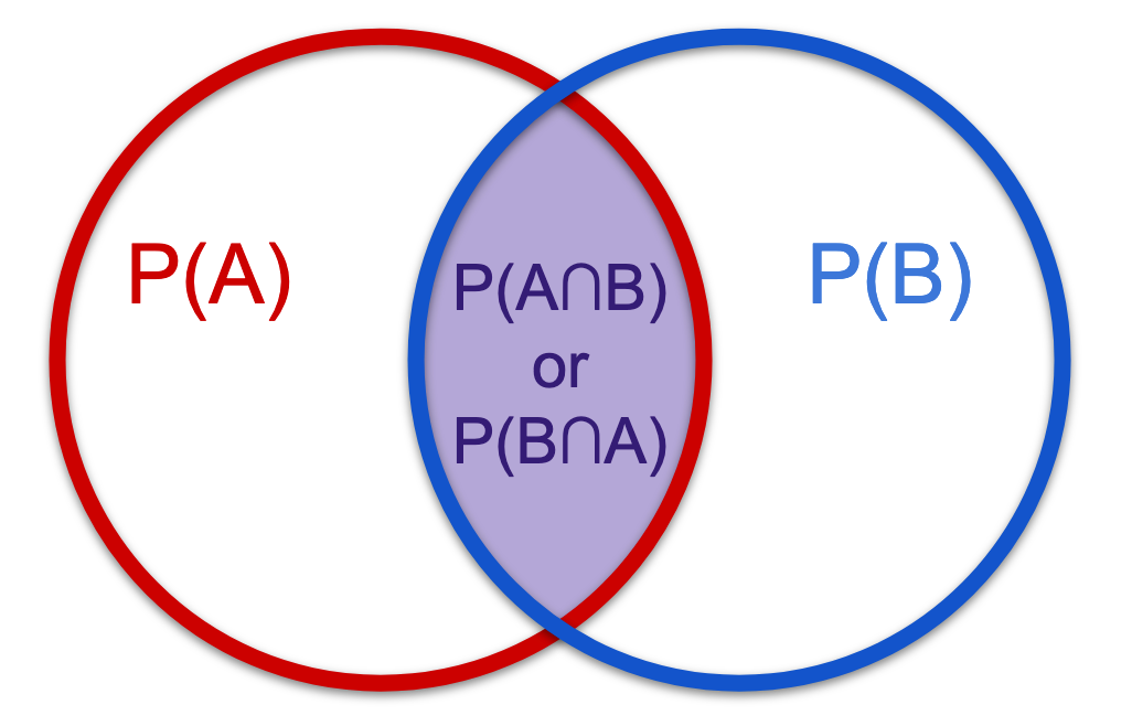
The shaded region is the intersection of both events happening together. The probability of A and B happening together, in turn, depends upon the probability of A or B happening at all, which is called the marginal probability. The marginal probability of the premise affects the probability of the conditional event. Marginal probability can even override the conditional entirely: All unicorns might have horns, but technically, if there are no unicorns, the probability of any given unicorn having a horn is zero, or rather, not defined (don't tell my daughter this, please).
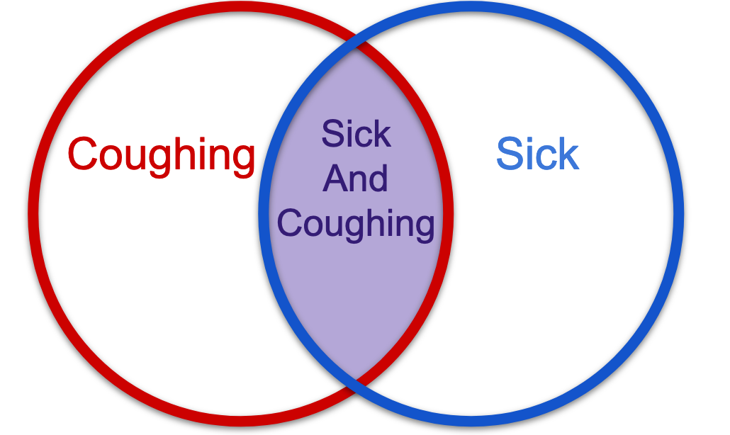
Marginal probability with a tangible example: Let's say you get a tickle in your throat. You cough once or twice. This is the Covid era, so immediately you wonder if this means that you're getting sick. "How worried should I be?" you ask yourself. Instinctively, you know that you need not be very worried, because there are a million reasons why people cough when they're not sick! Which is to say that your reasons for coughing while not sick are many, thus coughing is a weak an indicator of sickness (later, we will see that this instinct is the Bayes Factor, in mathspeak).
Normally you would not be overly worried about a cough. But a novel virus presents us with new, unknown, reasons to cough. With new reasons to cough come new marginal probabilities introduced into the equation. Since marginal probability is empirically derived, we do not have the rates, if we lack the data. But, of course, you don't want to wait for the data, only to find out after the fact that the data is much worse than you hoped. Probability is the language of being in "the world," which in turn, is a multi-dimensional horizon of possibility. What is normal changes, and your instincts about how worried you should be are suddenly outdated. "How much should I temper my worry?" you ask yourself.
In mathspeak, the formula for conditional probability is P(A|B) = P(B∩A)/P(B) per the Venn diagram (or commonsense). The probability of A happening, given B, is the probability of A and B happening together (the shaded overlapping region of the diagram), normalized by the probability of B happening at all. The premise, which has a marginal probability, is denoted by "given," and goes into the denominator, because it is that which the conditional term rests upon. We grant that B is the evidence, and only within the realm of B do we ask how likely A given be is. Vice versa for B given A (you may feel sick and wonder if you will start to cough).
The chance of you being sick, given that you are coughing, depends upon how often coughing indicates sickness, out of the many reasons to be coughing at all. Here, I write "at all" in bold, because it resonates a lot more with me than the word "marginal," or "regardless." Just remember that marginal means, "at all." The probability that your cough portends an oncoming sickness, depends upon how much of the total universe of coughing, is attributable to being sick. Hopefully by now, conditional probability makes total sense...
Bayes' Theorem is derived from conditional probability. And we are going to do the derivation right now, which is super exciting. But before we derive Bayes, let's take a look at the conditional probability formula one more time:
P(A|B) = P(B∩A)/P(B)
P(sick, given cough) is P(coughing while sick)/P(coughing at all)
Lets write the Conditional Probability equation a bunch of ways:
1) Given that I am coughing, what are the chances that I am sick?
2) What fraction of people who are coughing, at all, are sick people?
3) How indicative of sickness is coughing?
4) How much of the coughing universe consists of sick coughing?
5) What fraction of the entire B circle is the shaded region, A and B?
What if it's the other way around? You start to feel a little sick, and you wonder if this is going to turn into a full blown respiratory infection... Let's look at the Venn Diagram again. Clearly, it doesn't matter which side you approach the equation from, the intersection of B and A is going to be equal, right? However, intuitively speaking, you know that the chances of being sick just because you coughed, versus winding up coughing after you start to feel sick, are not the same.
That's because the classic Venn diagram is a fantasy, of course. Usually the two probability spaces are unequal. Sometimes very unequal. But even if the Venn Diagram looks like the one shown below, instead of the one above, the overlap stays the same, right? In other words, clearly you can approach the overlap from either direction, and it does not change. So even if P(A) and P(B) have totally different marginal probabilities, the region of the overlap remains the same in either expression.
This means that P(B|A) = P(A∩B)/P(A) or P(A|B) = P(B∩A)/P(B) both entail the same overlap, which is an important fact. But again, do not confuse this equal overlap with the idea that both versions of the equation are equal. These two equations will only resolve to an equality if you're ultimately dealing with a totally symmetrical Venn diagram. In the real world, the diagram will almost always look like this, that is, asymmetric:
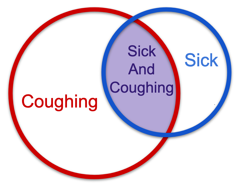
Again, in English: If you're coughing, there's a chance that you're sick. But it could be allergies, air quality, acid reflux, a crumb stuck in your throat, or a million other things. If you already feel sick, there is a better chance, I would think, of coughing. This obviously depends upon the main character of the story, too. This distribution of the probability space is just my hypothesis. I have not done the research, and often research will surprise you. For now, let's just assume that there is a much higher chance of coughing if you're already sick, than being sick just because you coughed, and that is because of the difference in marginal probabilities.
Deriving Bayes from Conditional Probability
In mathematics, wherever we can establish a theoretically certain equivalency, we have the opportunity to make substitutions and to derive new formulas! Substitutions are like money in the bank... So, let's isolate the known equivalent term of the equations, that is, the overlap: P(A∩B) and P(B∩A). We know these two terms are equal, because they are happening together. The overlapping region in a Venn diagram, just is, definitionally, the set of cases where both A and B happen together. This lets do the happy dance of moving the known puzzle piece to one side of both equations, and finally setting them equal to each other:
Step 1: P(B|A) = P(A∩B)/P(A) (conditional probability formula)
Step 2: P(B|A) * P(A) = P(A∩B)/P(A) * P(A) (eliminate denominator term)
Step 3: P(B|A) * P(A) = P(A∩B)
Now do the same for the other axis of the equation:
Step 1: P(A|B) = P(B∩A)/P(B)
Step 2: P(A|B) * P(B) = P(B∩A)/P(B) * P(B) (eliminate the denominator)
Step 3: P(A|B) * P(B) = P(B∩A) (P(A∩B) and P(B∩A) are equal as shown above)
Now we are ready to set the two different axes of the equation equal using a middle term:
P(A|B) * P(B) = P(A∩B) or P(B∩A) = P(B|A) * P(A)
Voila! There you have Bayes Theorem. Normally it's written with the middle term removed:
P(A|B) * P(B) = P(B|A) * P(A)
Here is how it is usually written, with the premise term (the given) moved into the denominator on other side:
P(A|B) = P(B|A) * P(A) / P(B)
Clearly, you can also write it like this:
P(A|B) = P(A∩B) / P(B)
Whether you're looking for A given B, or B given A, you can back into the information that you don't have, using information you do have. This becomes key when you attempt to make predictions about a population from a sampling. In theory, Bayes isolates the equation by which humans approach the world, learn from it, classify their experiences, and update their expectations. Clearly, such an equation almost cannot help but be useful. It's like the equation of use, qua use.
I hope you can now see that Bayes' Theorem is not different from conditional probability. To use a metaphor, it's as if Bayes realized that the marginal probabilities of any intersecting events render the conditional events to be expressed in different languages, and by extension, in different worlds. You can translate language A into language B, and you can translate language B into language A. While you may be saying the same thing, the words you will use will differ depending upon what is your desired language, and there isn't any reconciliation that gets you to the meaning itself. In this sense, Bayes gives us a convenient way to flip back and forth between worlds.
My Unique Version: The Shadow Venn
Understanding the derivation for Bayes is neat, but somehow it never helped me to solve actual Bayes math problems. Maybe it's my ADHD brain, but I used to go cross-eyed trying to figure out which was B given A, and which was A given B. I would try plugging values into the Bayes formula, get totally lost, and wind up doing what my high school math teacher would have called, "the plow horse method."
The plow horse method that I used was always to draw a probability tree, label all of the branches with probabilities. Then back into the trunk from the the terminal branches, multiply my way back out for each terminus, add up all of the relevant terminus probabilities, then find out what proportion of the relevant sub-branched my desired target represents. Wut?? Exactly! So work intensive and confusing. And most importantly, the plow horse method becomes untenable if your probability tree includes more than two or three layers of branches.
It did not help me that online tutorials for Bayes seemed always to jump from the derivation of Bayes Theorem, to talk of clinical trials and diagnostic tests, without any explanation for why this leap was happening, or why clinical trials and diagnostic tests became the chosen example. Like, why are we suddenly talking about test results for diagnosing diseases? I was still trying to figure out which is A and which is B, but suddenly the entire universe of YouTube tutorials is talking about test sensitivity vs. specificity?!? I feel totally lost!
After much reflection, I concluded that the reason Bayes tutorials resolve into examples that refer to diagnostic tests, is that it's really hard to ascertain the marginal probability of anything outside of rigorous controlled settings. Let's go back to the "Sick" and "Coughing" example. How would we ascertain the marginal probability of being sick? In other words, what are the chances of being sick at all? Or the marginal probability of coughing? It would be really really hard to know these. We would need to actually randomly sample a lot of sick and coughing people, right? We would need ways of testing them for being sick. We would need to make sure our sampling was truly random.
In pharmaceutical studies, all of the probability legwork has been done for you by scientists, which is why Bayes tutorials love using their diagnostic tests as examples. Clinical trials give us beautiful ready-to-use probabilities. From a clinical trial: You'll know the accuracy of the test, which is the probability that the test is positive when you're sick, and negative when you're not sick. These two numbers can even be different, as some tests are better at detecting sickness when it's present, than yielding a negative result when it's absent. You'll know the prevalence of the disease, that is, the marginal probability of having the disease at all. Given the prevalence, and the test accuracy, you can derive the rest.
How do we know the "accuracy" score of these tests? The test accuracy is derived empirically, in a grueling process in which diligent scientists looked at every single test subject who had a positive test in their trial, took a blood sample (or some other sample) and checked it under the microscope (or some other 100% accurate measure). From a large enough sample size, scientists are able to derive a highly accurate probability that their tests work (or don't work).
What I am calling the "Shadow Venn" represented by the dashed lines below, facilitates thinking about the transition from a Venn diagram, into a more useful version of the diagram. The traditional Venn diagram is deceptive, because it looks like there are only three main regions of concern. But there are two crucial realizations, which are left out: (1) The blank space outside of A intersected with B is a region as well, that is, neither A nor B. (2) Because A and B each, respectively, represent their own universe, the blank region outside of A and/or B is actually two differently shaped regions, superimposed.
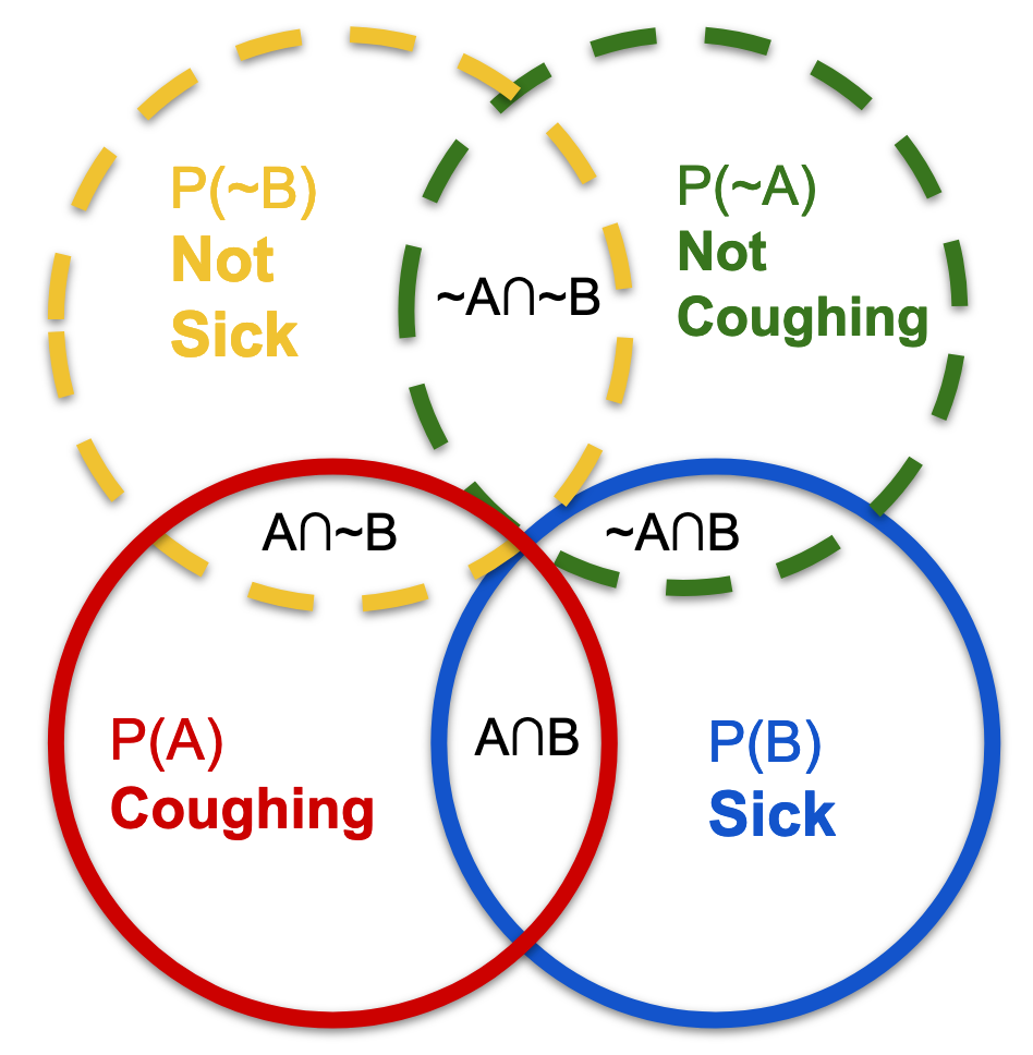
Thus, there are actually six regions of concern when it comes to solving conditional probability problems. These are (1) A, (2) B, (3) A and B, (4) neither A nor B, (5) the intersection of ~B with A, and (6) the intersection of ~A with B. Just like the marginal probability of A might be very different from the marginal probability of B, the probability of not-A might within B might be very different from not-B within A, however this difference is not obvious in the traditional Venn diagram. You need the Shadow Venn, which I invented, in order to clearly see the distinction.
I like to think about the "negative space" within a Venn diagram as having two axes. There is the A-axis, when you approach ~B with respect to A. And there is the B-Axis, when you approach ~A with respect to B. Without the Shadow Venn to reference, I would find this explanation totally inscrutable. It's already pretty confusing to talk about, without simply pointing to the diagram that I drew. However, I find the idea of axes to be especially helpful, because of how it invokes vector math, and ultimately matrices. The idea that each conditional is a transformation of a premise, will be key to grasping more complex Bayes problems.
If axes do not help you, perhaps nodes and worlds will. Let's say that each node on a probability tree represents the forking of one universe into two or more other universes. Considered in this light, it's not difficult to see how the Shadow Venn comes into play. In the traditional Venn, you only have a blob for A: Coughing. Whereas, in a probability tree diagram, the A node, which is the first node, already includes a fork into A and not-A. From there, further forks can occur, such as B and not-B. In a probability tree, it becomes clearer that there are more dimensions to the problem, which need to be taken into account.
In another blog post, I go through a more complex probability tree, and show how to understand it using vectors [INSERT LINK HERE].
A Classic Bayes Example: Diagnostic Tests
So you take a diagnostic test for some horrible disease, and you test positive. OMG. How worried should you be? In other words, the question that is tearing up you mind is this: Given that I tested positive, what is the probability that I have the disease? Well, it depends how accurate the test is, right? Yes. But it also depends on how likely you are to test positive even when you don't have the disease. You are now in the universe of people who tested positive. And what you really need to know is what proportion of the positive test universe is truly positive.
Let's rehearse a fully fleshed out example:
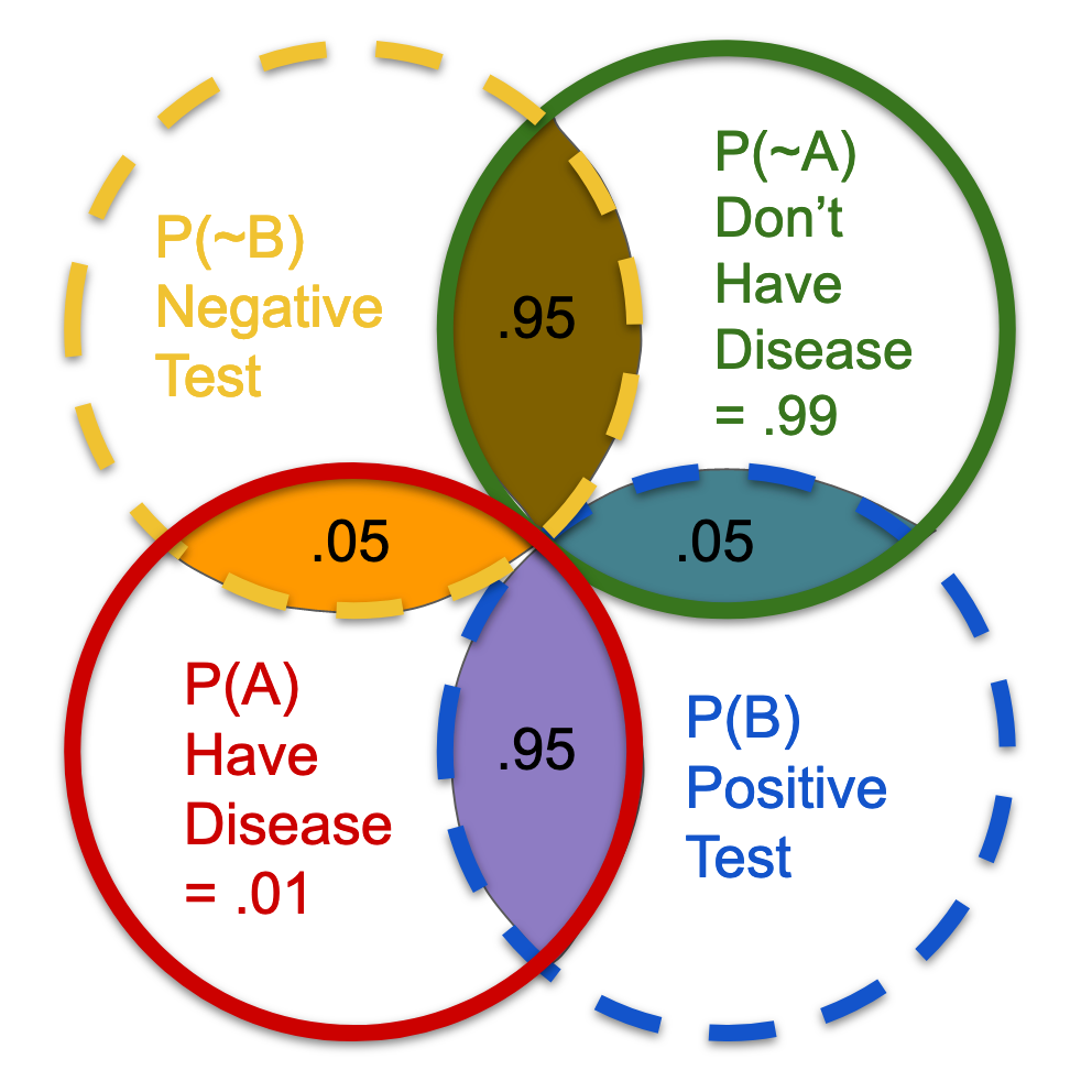
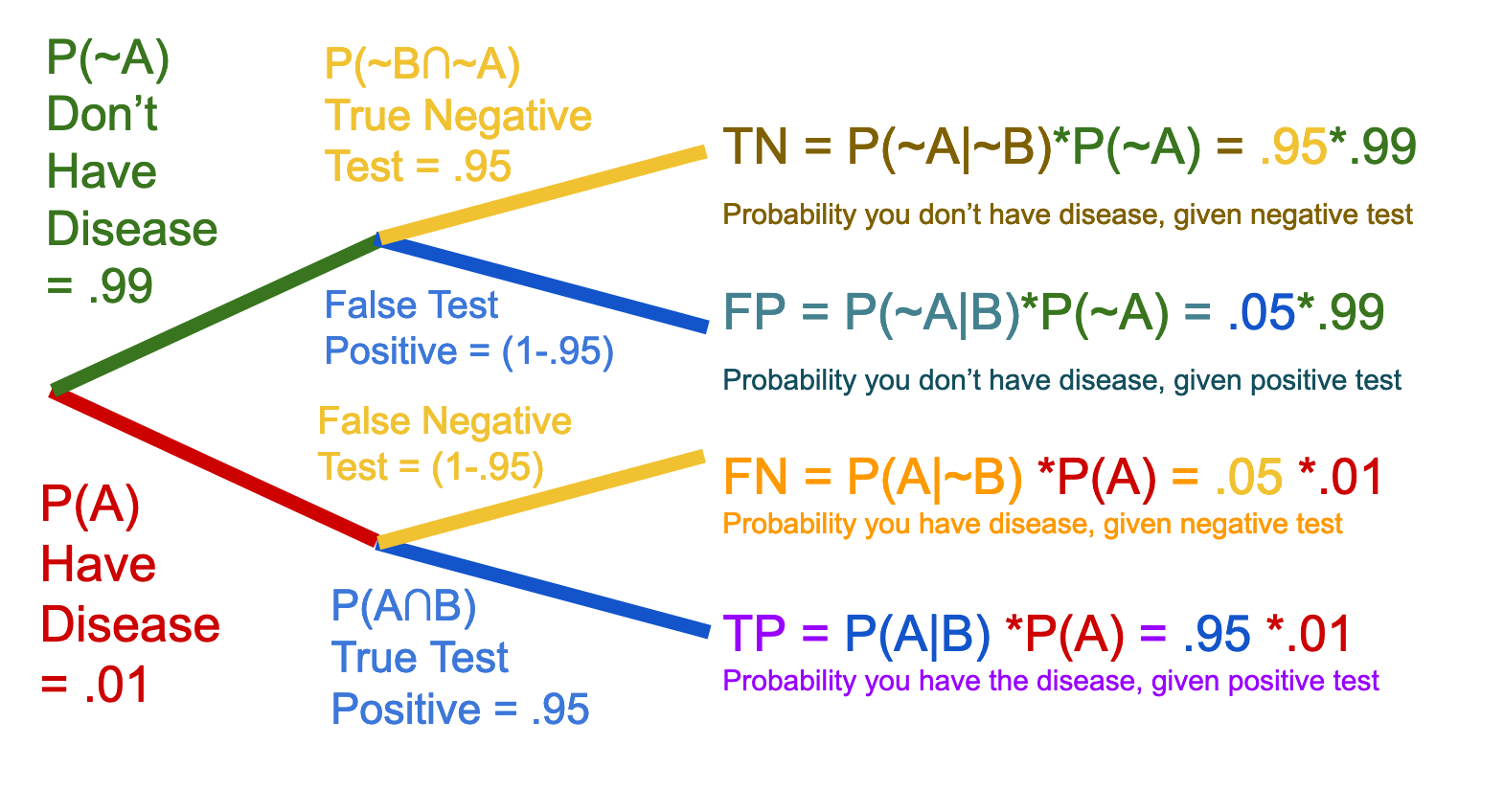
Prior to administering tests, we know that the prevalence of a disease is about 1%. Assume that scientists have arrived at this number via random sampling. Having the disease versus not having it is a binary, so the prevalence number gives (1 - .01)= 99% of people do not have the disease. We also know that the diagnostic test is 95% accurate. For the sake of simplicity, we are not further qualifying the accuracy number into sensitivity vs specificity. We assume that 95% accuracy means that the test finds 95% of disease when it is present (but misses 5% in a false negative). Conversely, it generates a true negative result for 95% of people who don't have the disease (but gives a false positive rate of 5%).
P(A|B) = What we want to know: Chance of having disease, given positive test
P(B|A) = .95 Test accuracy: Chance of testing positive, given you have disease
P(B|~A) = .05 Test inaccuracy: Chance of testing positive, given you have no disease (derived from test accuracy *not always 1-accuracy!!!)
P(A) = .01 Disease prevalence: probability of having the disease, at all
P(B) = .99 Probability of not having the disease, at all (derived from P(A))
If you get nothing else out of reading this post, just remember that the Bayes formula always puts the premise in the denominator. Whatever follows "given" goes in the denominator. Why? Because that is the marginal probability, upon which the conditional rests. Given a positive test result means that we are situated in the universe of positive test results, and ultimately we want to know what portion of those positive test results are, in fact, positive. This means that the false positive results will play a major role.
In the following section, I will complete this example using a Shadow Venn and a probability tree. The marginal probability of the axis of the question, in this case, testing positive at all, which always trips me up when I attempt a Bayes question using a probability tree. You have to fetch or round up the false positives from the not-Disease branch, which is counter-intuitive. For a test that is 95% accurate, it feels intuitively like the probability of testing positive should be 95%. But that is not the case! Just because you took a super accurate test, and it's positive, doesn't mean you have the disease! Of course, you should be concerned, but don't freak out!
*Test accuracy can come with an added dimension whereby true and false test results are not a direct inverse of each other, as they are in this example. In other words, a text might be 99% accurate in identifying true positives, i.e. detecting sickness when it is there, but only 90% accurate in terms of true negatives, i.e. not accusing when disease is lacking. For the sake of this example, we keep it simple and have a singular accuracy number, which is not further qualified as in test sensitivity vs. specificity, the former being the sensitivity to true positives.
Reënvisioning Bayes
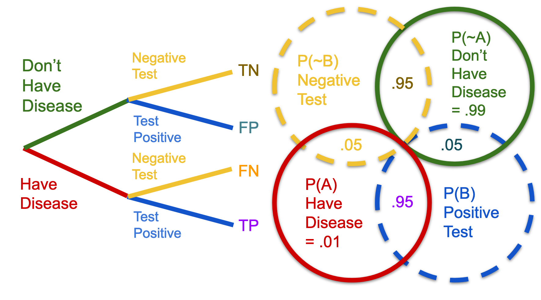
The Probability Tree diagram and the Venn diagram need not be considered two different diagrams, but two perspectives on the same diagram. The Shadow Venn shows the additional dimension, which is added to the initial A~A node, which is not readily obvious in the traditional Venn diagram.
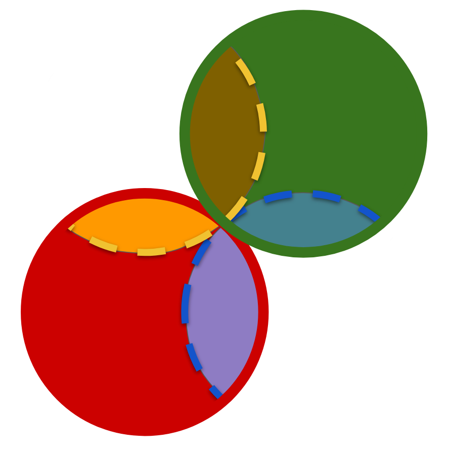
Picture the probability tree on the left below as a three dimensional tree, with translucent (perhaps fiber-optic) colored trunks and branches. The main trunk is your first Venn diagram layer. The branches are the second layer, which is represented by the Shadow Venn, shown in the Venn below with dashed lines. The overlap regions represent the smallest, terminal branches.

Below is what the tree might look like, if observed from above. You've got the two main trunks, which are the red and green circles. The mixed colors of each terminal branch indicates the trunk, of which each type of branch is an offshoot. Because the trunk and branches in our thought experiment are colored fiber-optic, the colors mix together. The shaded regions represent the terminal branches of the probability tree.
If you are still not seeing it, try the version of the drawing below... If you have the disease, you either test negative for it, or you test positive for it. Thus, there is no region in the second tier of branches, which falls outside of the overlap with the first tier. I tried to show this using the dashed lines in the previous drawing, however, it may be easier for folks to visualize without those regions erased, as shown below.
Simply put, branches branch off of trunks, so there are no trunkless branches. However, there are obviously a ton of people with or without the disease in the overall population, who have not taken the test. Thus, when you get a test result, you still need to normalize your overlap region with the marginal probability of the relevant trunk. The trunk is your premise, your "given," in other words, and all aspects of it need to be factored into the denominator.
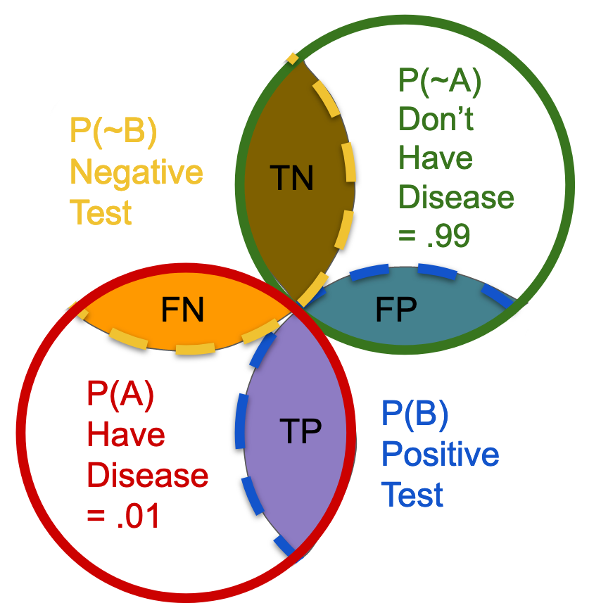
The most important point to takeaway from this visualization exercise is this: When asked, "Given a positive test, what are the chances of having the disease," you are only concerned with the blue branches, i.e. the positive test branches. One really simple way to write the equation, which corresponds to this question is as follows: True Positives/All Positives, or TP / TP + FP. In the universe of all positive results, how many of those are true positives?
While probability trees usually get me to the desired answer, someway somehow, they can be really confusing. I think the main source of the confusion comes from the order of the premise. If you recall, what we aim to solve is P(A|B), which is the probability of having the disease, given the positive test result. However, when it comes time to draw the tree, you are drawing the tree for the right hand side of the equation, which begins with the inverse, P(B|A). Thus, the premise gets inverted in the tree form. Rather than starting with, "Given a positive test result," the tree structure begins with, "Given that you are sick..." And you can see that the first node is in fact the [A ~A] node.
When I used to do the plow horse method, what I was really doing was retrieving the marginal probabilities: The trickier one of testing positive at all, but also the disease prevalence rate. Converting the probability tree from the plow horse method into a mental multi-tiered Venn diagram, it helps me sort in my mind which region is of primary concern to the question being asked, and it ultimately helps me rephrase the question into something I can wrap my head around.
I was essentially taking a Bayes' problem, and forcing it to resolve as a frequentest problem. This is a totally legit way to solve the problem. It just takes more work, and it's not practical for more than a few dimensions...Having visualized the tree, and its relationship to the Venn diagram, let's go back to diagram:
If we know the test is 95% accurate for folks who have the disease, what can that tell us about the chances of testing positive at all? Well, it means that if you are not sick, 5% of the time, the test is going to miss that. And that is a HUGE number of people, right? Because, according to our empirical data, thats 99% of the entire population. So, the probability of testing positive when you are sick is a large percentage of a tiny number; but the probability of testing positive when you aren't sick a tiny percentage of an enormous number (99% of the population).
P(A|B) = What we want to know (chance of disease, given positive test)
P(B|A) = .95 test accuracy (known)
P(B|~A) = .05 test inaccuracy (derived from test accuracy)
P(A) = .01 disease prevalence: probability of having the disease, at all. (known)
P(B) = .99 probability of not having the disease, at all (derived from P(A))
So let's plug it all in and see what we get:
P(A|B) = P(B|A) * P(A) / P(B)
P(A|B) = .95 * .01 / P(B)
P(B) = Probability of having the disease at all = True positives + False Positives
P(B) = TP + FP
FP = Positives missed (100% minus test accuracy)*(% of people who don't have disease)
P(A|B) = .95 * .01 /(.95 * .01) + ((1 - .95)(1 - .01))
P(A|B) = .0095/.0095 + .0495 = .0095/.059 = 16.10%
16% chance. You have a 16% chance of actually having the disease, if you test positive for it. Why is that? Well, it's because, really your probability space looks more like this (not intended to be perfectly to scale, also please forgive minor overlap fails, as I drew all of these diagrams in Google Slides, which is not a drawing program):
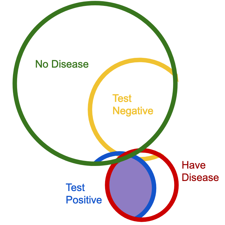
Clearly the shaded region, which we are seeking, which is the purple area, is a small portion of the overall possibilities, which lines up with the result of our calculations.
Matrices as Trees
At some point, when I was envisioning different ways of relating Bayes schemas, it occurred to me that probability trees can be converted into matrices, just as well, or better, than they can be converted into stacked Venn diagrams.
If you think of the first level of a probability tree as a 2x1 matrix (which is a vector technically), and you think of the second layer of the probability tree as another 1x2 matrix (or vector), then your four resulting options are going to represent your possible probability permutations, and the numbers will go right along with them. The other interesting thing about the matrix formation is that it's really easy to see the axes of your marginal probabilities. Clearly the marginal A axis is the vertical axis, and the marginal B axis is the horizontal axis.
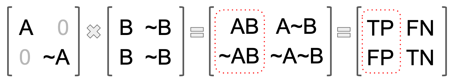
Probably a really smart mathematician would be like, duh, the probability table is just a sketch of a bunch of vectors transformed by other vectors, so you're really just making a tautological claim here. Or maybe a really smart mathematician would pat me on the head for this. I have no idea.
More on this in our discussion of the Odds Form of Bayes
What is the point of Bayes?
So, if you can only solve Bayes problems when you have access to probability data, which is basically impossible to get outside of a laboratory, what is the point of Bayes? Other than solving narrow esoteric word problems about diagnostic tests and defective factory widgets, what is it for?
What Bayes does is mimic the logic of human decision making, which is why it forms the basis of "machine learning," now often called "AI."
So, take the Sick|Coughing example. That was obviously a huge oversimplification. When you're sitting there wondering if you might be getting sick, you're not just thinking about your cough. Really, your mental math is much more complex:
P(Sick|Cough+Allergies+Fever+Mucus+Air_Quality+Sick_Kid...)
When you as a human are trying to learn and decide things, you're taking into account an entire vector of contributing factors. Not only that, but you are a super dynamic model; you update your expectations as you notice the contributing factors change, and the marginal probabilities change. In the next post, we are going to look at Bayes with multiple data dimensions.
In another post, we look at different ways to compute multiple parameters in the premise, and examine a more complex tree! [INSERT LINK HERE]