Your Own Personal Loss Function
Every Data Scientist should be able to conceptualize a dataset as a matrix, even if you never touch a matrix in your life.
For me, heaven is a place where I can take every mathematics class that Professor Gilbert Strange ever taught. Most of the time, I find the pedestal narratives applied to professors at big research universities to be farcical. Why? In graduate school at UChicago, I found many of the tenured professors (who shall remain unnamed of course) to be pompous and not only uninterested in teaching, but actually contemptuous of it. Not Gil Strang, though. Gil Strang wanted to teach, and did it well. He deserves to be lionized, misogynistic jokes about Monica Lewinsky notwithstanding (it's a fallen world, after all). Last year, Professor Strang gave his final lecture. I expect he will not even know what a legend he truly is until Judgment Day.
With good math teachers, I am really good at math. Without good teachers, I flounder. Which is why I am so grateful for Gil Strang. Because of him, I actually understand Linear Algebra now, when I did not understand it in high school. The anorexia and panic attacks didn't help, but the mediocre math teacher certainly did not help. Perhaps it was not the teacher's fault. Back in the 1990s, Linear Algebra was not as exciting a field. Things changed when processors changed. Better late than never, though; both for the entire discipline in mathematics, and for myself as a student thereof. Matrices are everywhere now, and they power everything in Machine Learning and AI. Without matrix math, there would be no computers, no Google, no Tesla, no ChatGPT...
How did I stumble on Gil Strang as a philosopher? Well, a couple years back, in the depths of new motherhood and a global pandemic, I decided to take an Applied Data Science course, in which Mathematics for Machine Learning was assigned reading. Mostly, I took the course because I felt impotent in terms of assessing statistical information. The worst vice is advice, and let me tell you, new parents are inundated with well-meaning advice. New parents during a pandemic, I would hypothesize, are the cohort most subjected to unsolicited science-sounding advice, in the history of the universe. I did the assigned reading, and while a lot of it was over my head, in a footnote, I found a reference to Gil Strang's legendary 18.06 Linear Algebra course, which to my utter delight, was (and is) available for free, online through MIT OpenCourseWare. I absolutely gobbled it up.
These days, the world is awash in DS certs and bootcamps. Now that ZIRP (zero interest rate policy) is over, tech has gone a bit soft, and the envious are coming out of hiding to make fun of bootcamp people. Mine was a six-month course, and while I cannot speak for other bootcamps, I have zero regrets. To the contrary, I am so glad that I chose a course with a math prerequisite exam, and specifically, a course that led me to discover Gil Strang. I got a 50% Covid discount on the tuition fee, but I would have been more than happy, had I paid the full price.
Learning to think in matrices is essential to becoming a Data Scientist. In this essay, I am going to attempt to explain statistical modeling, by reference to the classic concept of Linear Regression. First, I am going to introduce the idea of a dataset as a system of equations. Then I am going to compare the old and cumbersome Calculus way to the elegant and beautiful Linear Algebra way of deriving a loss function that best fits the data in the data set. While I am using the example of regression here, it applies to other models. Even if you never touch a matrix in your life, you should be able to conceptualize a dataset as a matrix. Models of all kinds rely heavily on matrix operations for embedding representations and performing transformations.
Life Is an Underdetermined System of Equations
In applied math, systems of equations rarely or never have a definite solution. Why? Because observable data points scatter themselves every which way, and any model that attempts to fit the data is doomed to be imperfect ("doomed" is ironic here). In other words, the model is the best solution, in the absence of a perfect solution. The model will be a line, a plane, a hyperplane, a polynomial, a support vector... any number of lines, squiggles, or hyper-objects in multi-dimensional space, which come as closely as possible to each and every data point, without necessarily touching any of them.
The intended audience here is the uninitiated. People who, like me, did not study math in college. You, the reader, may find my goal to be unrealistic and pointless. If nothing else, trying to explain matrices like you are five will be good practice for the day when I become my own children's linear algebra tutor. If you have the ability to grasp the formula for a line–good old y=mx+b then you can understand Ax=b, since the latter is just a compilation of the former. Do not be confused by the "b" terms. These do not mean the same thing. The point is that in a multiple regression analysis, each x gets multiplied by a weight, and added up together, to give a best-fit solution.
In matrix-speak, the systems of equations, which everyday life yields, are rectangular. Think Excel spreadsheet, if you have no experience with databases. In a typical spreadsheet, there are only a few columns, and potentially hundreds of thousands of rows, or vice versa. Geometrically speaking, in any case, the array structure is a rectangle. If every matrix with a definite solution is square, then we know ahead of time that real life datasets are under-determined, i.e. rectangular. In a rectangular system, row reduction resolves into pivot variables yes, but also a bunch of free variables, which can be assigned values, but do not inherently have them. The ultimate solution vector, by extension, contains degrees of freedom, which I interpret to mean that it's up to us to populate them. Freedom, after all, is a responsibility.
Of course, I am being a bit glib and facile here. Real-life data could come in a square array, but it would in all likelihood be square in appearance only, i.e. a rectangular matrix masquerading as square. A lot of square matrices reveal themselves to be actually rectangular matrices, consisting of informative columns, and redundant ones. It's the redundant ones that cause trouble... The point is that we can arrange any data set into a system of equations, by imagining each explanatory variable as being a matrix of weights or coefficients, which when combined, result in the set of Y variables. And we can conceptualize any loss function as the vector of x values, which when multiplied by the coefficients, results in the set of target variables.
On the other hand, the perfect matrix, which represents a system of equations, with one and one solution only, is square. The solution vector in a system of linear equations Ax=b, which has a definite solution, can be thought of as analogous to the best-fit line or plane in a regression model, except that it exactly intersects every response variable. Again, this matrix is inherently square, and resolves perfectly to reduced row echelon form. In practice, this never ever happens. In fact, there is nothing more terrifying to a Data Scientist than a model that fits 100% of the data, since that means there is data leakage somewhere in your code.
Generating a "best fit" model is not as easy as it sounds. Geometrically speaking, drawing a model is easy. Most people can eyeball a best-fit line or curve. However, generating the equation of that model is another story. A model is supposed to come as closely as possible to every observed data point, which means that the measure of fitness is the distance between the model and the data. Anyone who has ever touched a statistical regression problem must have a good feel for the daunting chasm between theory and practice. In regression it becomes obvious that achieving the model equation means solving as many equations as there are data points, simultaneously.
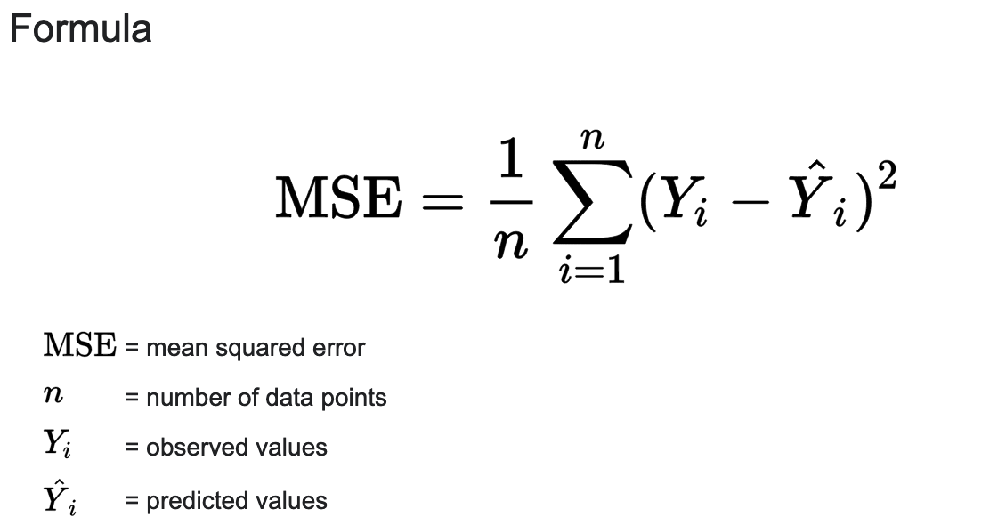
Least Squares is the most used method in statistics to perform linear regression. Enter State Right: The Loss Function.
Below you will find the formula for Mean Squared Error, which is the function that most often gets "minimized" in least squares. The difference in Y terms, Y vs Ŷ, just is the difference between the model output and the observed data. Luckily, whenever minimization is desired, the math gods have given us a well stocked toolbox, with which to force the formula, as it were, and make it approach zero. The two main choices from Calculus, and more recently, Linear Algebra.
Data comes in many patterns, and may not be adequately modeled with linear functions. For nonlinear cost functions, there are other methods for minimization, such as gradient descent. In this post, we will deal only with linear data.
The Calculus Way
In Calculus, the first derivative is the instantaneous rate of change of a function. Wherever rate of change goes to zero, the original function, (of which the derivative is derived), reaches an inflection point: A hill or a trough, a maximum or a minimum. The MSE function produces only positive values for the coefficient of the squared term, which means it's convex. Thus, wherever the first derivative goes to zero, you can be sure you will find the coefficients for your model, because those will be the weights, which when applied to any x, will produce the smallest possible y. By this method, we back into our model via the solution set. Hence "regress."
"Just take the first derivative of the loss function and set it to zero, and voila! You have your model!" Sounds great, but computationally, the Calculus version is hell, especially with multiple coefficients (for multiple independent variables). In the robust parametrized models of modern data science, there are literally thousands of independent variables. Each and every variable requires taking a partial derivative with respect to its respective coefficient, then setting the resulting function equal to zero. That is a lot of hairy math!
The math is so hairy, in fact, that it's tough to find any instances where an instructor actually slogs through the computations. Usually instructors compute partial derivatives, and end with hand waving and assurances that software that will do the computations for you... And if you care to go through the computations below, you will find out why. The funniest thing about the Calculus formula is that it resolves into a matrix at the last step. It resolves into the matrix, which constitutes Step 1 of the Linear Algebra methods. That's right! You can't even do Calculus without Linear Algebra. So why leave the reservation in the first place? Obviously, I am kidding. But every joke contains some kernel of truth.
Jump to "The Linear Algebra Way" to skip over the Calculus computations.
Let's go through the steps of using Calculus to compute a fairly simple linear regression model (with two parameters):
I. Define the Multiple Linear Regression Model:
Ŷ = β0+β1X1+β2X2
where:
- Ŷ is the model (predicted values).
- X1 and X2 are the independent variables.
- β0 is the y-intercept.
- β1 is the coefficient for X1.
- β2 is the coefficient for X2.
II. Minimize the MSE with Respect to β0, β1, and β2:
Now that we have defined the model function, we can plug it into the loss function (in this case the MSE), and "optimize" it. To minimize the MSE, you need to find the values of β0, β1, and β2, which make it equal to zero at the respective first derivative. To do this, you set the partial derivatives of the MSE with respect to each coefficient (β0, β1, and β2) equal to zero. (Note that every ∑ summation term below is a sum to n with interval 1. In some cases, I have simplified the notation.)
1. Partial Derivative with Respect to β0:
∂/∂β0 (1/n ∑i=1 (Yi− (β0+β1X1i+β2X2i))2) = 0
2. Partial Derivative with Respect to β1:
∂/∂β1 (1/n ∑i=1 (Yi− (β0+β1X1i+β2X2i))2) = 0
3. Partial Derivative with Respect to β2:
∂/∂β2 (1/n ∑i=1 (Yi− (β0+β1X1i+β2X2i))2) = 0
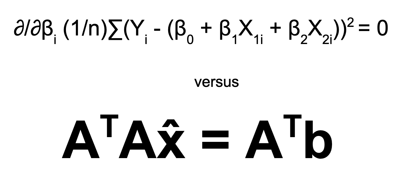
Maybe this doesn't look so bad to you, but we have only just written out formulas. In order to solve them, we need to do a lot of algebra. In what follows, I will go through the actual steps of solving... Once we take all of these partial derivatives, you will see that the resulting system of equations, sometimes called "the normal equations," resolves to be the same linear system as ATAx̂=ATb. Yes, the MSE is quadratic, but its derivatives are linear with respect to the weights.
Note that we don't really need the 1/n part of the MSE equation. For the purposes of our equation, 1/n is a constant, because n is a known variable. It is not one of the unknowns, which our equation aims to solve. Any constant can be factored out of all terms of a summation–and in the context of setting the equation equal to zero, can be cancelled out if desired. It's good to know that it's there, and of course, it in some ways is a very important number. "Sum of Squares," the non-normalized cousin of MSE, is basically the same thing as MSE, except not averaged, i.e. not divided by n.
Alright, let's keep plugging away:
IIIa. Take a partial derivative with respect to β0 (Note: All ∑ notation is ∑i=1 summed to n):
OK, so we start with the MSE equation, which again, is our loss function:
MSE = (1/n ∑(Yi - (β0 + β1X1i + β2X2i))2)
Let's compute the derivative and set it equal to zero. Here you may be tempted to expand the squared term (Yi - (β0 + β1X1i + β2X2i))2, but don't do it! It's much easier to use the chain rule. Bring down the exponent down into a leading constant, and derive the inner function. Thus the derivative simplifies as follows:
∂/∂β0 (2/n) ∑(Yi - (β0 + β1X1i + β2X2i)) * (-1) = 0
Next, you can get rid of 2/n by multiplying both sides by its inverse. Then multiply through with the -1 derivative term:
∑(Yi - β0 - β1X1i - β2X2i))* (-1) = 0
First, we distribute the minus sign inside the parenthesis above. Make sure you get your signs right! We don't want to make a negative/positive signs error. (I made a sign error while preparing for this post, even though I tried hard not to):
∑(-Yi + β0 + β1X1i + β2X2i) = 0
Now, we want to isolate all components of the equation, which are subject to summation. These isolated components will result in modular building blocks, so to speak, which are easier to work with. In other words, we move the ∑Yi term out, followed by the other terms.
-∑Yi + ∑β0 + β1∑X1i + β2∑X2i) = 0
The y-intercept β0 ultimately is a constant. Therefore, the sum of all β0 is just n*β0. Similarly, the coefficients β1 and β2 will be constants, which means they can be moved in front of their summations.
-∑Yi + nβ0 + β1∑X1i + β2∑X2i = 0
The final step of this calculation, once we draw the partial derivatives for the other two variables, will be to organize all three equations in a linear system. In order to do this, we will want all of the equations in the form of β0+β1+β2=Yi as shown:
∑Yi = nβ0 + β1∑X1i + β2∑X2i
Let's keep this equation on the back burner, while we work on the other two coefficients' partial derivatives. Also, just to note, we can bring back the 1/n if we want. Not needed at the moment.
IIIb. To take a partial derivative with respect to β1, you follow these steps (all ∑ notation is ∑i=1 summed to n):
The MSE equation is (the same as the equation we started with above):
∂/∂β1 (1/n ∑(Yi - (β0 + β1X1i + β2X2i))2) = 0
Let's compute the partial derivative and set it equal to zero, like we did before. Again, using the chain rule, the derivative simplifies as follows:
∂/∂β1 = (2/n) ∑(Yi - (β0 + β1X1i + β2X2i)) * (-X1i) = 0
Once again, we can get rid of the 2/n because it's just a constant, and we can multiply both sides by its inverse. We can always bring it back later if we want:
∑(Yi - β0 - β1X1i - β2X2i)) * (-X1i) = 0
Distribute the -X1i term from the outer parenthesis, multiplying each term inside the parenthesis by the X1i term.
∑(-YiX1i + β0X1i + β1X1i2 + β2X1iX2i) = 0
Distribute the summation terms. Then, factor out the constant terms for each summation component.
-∑YiX1i + ∑β0X1i + ∑β1X1i2 + ∑β2X1iX2i = 0
As before, we want to organize the terms so that we can easily put them into a matrix of linear equations at the last step. It may help to realize that the X and Y terms are not variables, which we need to solve for. Values for those terms will be given by the data points we have. We are solving for the coefficient terms β0, β1, and β2.
∑YiX1i = β0∑X1i + β1∑X1i2 + β2∑X1iX2i
IIIc. To take a partial derivative and solve the first equation for β2, you follow these steps (again all ∑ notation is ∑i=1 summed to n):
OK the MSE equation again: ∂/∂β2 (1/n ∑(Yi - (β0 + β1X1i + β2X2i))2) = 0
Let's compute the derivative and set it equal to 0:
∂/∂β2 (1/n ∑(Yi - (β0 + β1X1i + β2X2i))2) = 0
Using the chain rule, the derivative simplifies as follows:
(2/n) ∑(Yi - (β0 + β1X1i + β2X2i)) * (-X2i) = 0
Now, you can move 2/n out of the equation by multiplying both sides by n/2. Then distribute the X term:
(2/n) ∑(Yi - (β0 + β1X1i + β2X2i)) * -X2i = 0
∑(-YiX2i + β0X2i + β1X1iX2i + β2X2i2) = 0
As before, distribute the summation. Remember that all β terms are constants, so they can be moved in front of the sigma:
-∑YiX2i + β0∑X2i + β1∑X1iX2i + β2∑X2i2 = 0
Now, isolate the term containing Yi on one side:
∑YiX2i = β0∑X2i + β1∑X1iX2i + β2∑X2i2
IV. Now we can arrange our three equations into a system of linear equations, and given some data points, we have everything we need to solve for our coefficients.
∑Y = nβ0 + β1∑X1i + β2∑X2i
∑YX1i = β0∑X1i + β1∑X1i2 + β2∑X1iX2i
∑YX2i = β0∑X2i + β1∑X1iX2i + β2∑X2i2
These equations are very cool. You will see why in a bit.
The final step in the calculus version is to take some sample data points, and plug them into the equations above. Then use row reduction to solve the system. Example Data:
- (x1₁, x2₁, y₁) = (2, 1, 4)
- (x1₂, x2₂, y₂) = (3, 2, 5)
- (x1₃, x2₃, y₃) = (4, 6, 7)
- (x14, x24, y4) = (5, 4, 5)
First, we need to compute the values for the right-hand sides of these equations using the provided data:
Let's calculate the sums for each variable:
- Number of data points (n) = 4
- Sum of the dependent variable (Y):
∑Y = y₁ + y₂ + y₃ + y₄ = 4 + 5 + 7 + 5 = 21 - Sum of the first independent variable (X₁):
∑X₁ = x1₁ + x1₂ + x1₃ + x14 = 2 + 3 + 4 + 5 = 14 - Sum of the second independent variable (X₂):
∑X₂ = x2₁ + x2₂ + x2₃ + x24 = 1 + 2 + 6 + 4 = 13 - Sum of the squares of the first independent variable (X₁²):
∑X₁² = x1₁² + x1₂² + x1₃² + x14² = 4 + 9 + 16 + 25 = 54 - Sum of the product of the first and second independent variables (X₁X₂): ∑X₁X₂ = x1₁ * x2₁ + x1₂ * x2₂ + x1₃ * x2₃ + x14 * x24 =
(2 * 1) + (3 * 2) + (4 * 6) + (5 * 4) = 2 + 6 + 24 + 20 = 52 - Sum of the squares of the second independent variable (X₂²):
∑X₂² = x2₁² + x2₂² + x2₃² + x24² = 1 + 4 + 36 + 16 = 57 - Sum of the product of the dependent variable and the first independent variable (∑YX1i): ∑YX1i = (y₁ * x1₁) + (y₂ * x1₂) + (y₃ * x1₃) + (y4 * x14) =
(4 * 2) + (5 * 3) + (7 * 4) + (5 * 5) = 8 + 15 + 28 + 25 = 76 - Sum of the product of the dependent variable and the second independent variable (∑YX2i): ∑YX2i = (y₁ * x2₁) + (y₂ * x2₂) + (y₃ * x2₃) + (y4 * x24) =
(4 * 1) + (5 * 2) + (7 * 6) + (5 * 4) = 4 + 10 + 42 + 20 = 76
Now, we can substitute these values, as "modular components" into the normal equations:
nβ0 + β1∑X1i + β2∑X2i = ∑Y
β0∑X1i + β1∑X1i2 + β2∑X1iX2i = ∑YX1i
β0∑X2i + β1∑X1iX2i + β2∑X2i2 = ∑YX2i
- 4β0 + 14β1 + 13β2 = 21
- 14β0 + 54β1 + 52β2 = 76
- 13β0 + 52β1 + 57β2 = 76
Nice! Now all we need to do is put these numbers into a matrix, and row reduce, or LU decompose, and solve for β0, β1, and β2.
The Linear Algebra Way
If you are like me, you dislike sigma notation, ∑. Granted, there is an element of personal bias in my memories of first encounters with sigma. Summations marked the beginning of the end for me, in high school. This had nothing to do with math. Rather, I couldn't hear myself think over the sound of the angels screaming, so to speak, and I remember sigmas being among the flotsam swirling in the dark and roiling waters, in which my soul nearly drowned. But now I am back, and I don't mind sigma notation. However, if I can avoid it, I would rather avoid it.
Probably my favorite thing about Linear Algebra, is that summation is built into matrix operations, which frees us from the need for the scary-looking sigma notation... Summation is built into the matrix of matrices, as it were. In other words, summation is a default matrix operation, so we don't need the sigma notation. Linear algebra formulas for least squares eliminate the annoying sigma notation, but perhaps even more joyously, they make added data dimensions really simple to compute. The same formula that works in one dimension works in three, twelve, and thirty thousand dimensions. I don't want to look at the Calculus version with 30,000 x-variables. Perish the thought!
Here it is, the linear algebra formula for Least Squares:

Isn't it beautiful? I honestly want to get a tattoo of this formula. All you need to solve it are two things, which in any data project, you are sure to have: (1) Your x-values, arranged in an array; and (2) your y-values, (the predicted values), arranged in a vector, appended to the array. That's it! The Fundamental Theorem of Linear Algebra gives us this beautifully elegant least squares formula, and it works for any system of linear equations (any matrix). If you are interested, I derive the formula in the next section of this post.
In the Calculus version, once we take all of the requisite partial derivatives, the resulting system of equations, sometimes called "the normal equations," resolves to be the same linear system as the system of matrices generated by the linear ATAx̂=ATb. It's pretty amazing how that works.
So, let's pretend that we have the same data points from the Calculus example above:
- (x1₁, x2₁, y₁) = (2, 1, 4)
- (x1₂, x2₂, y₂) = (3, 2, 5)
- (x1₃, x2₃, y₃) = (4, 6, 7)
- (x14, x24, y4) = (5, 4, 5)
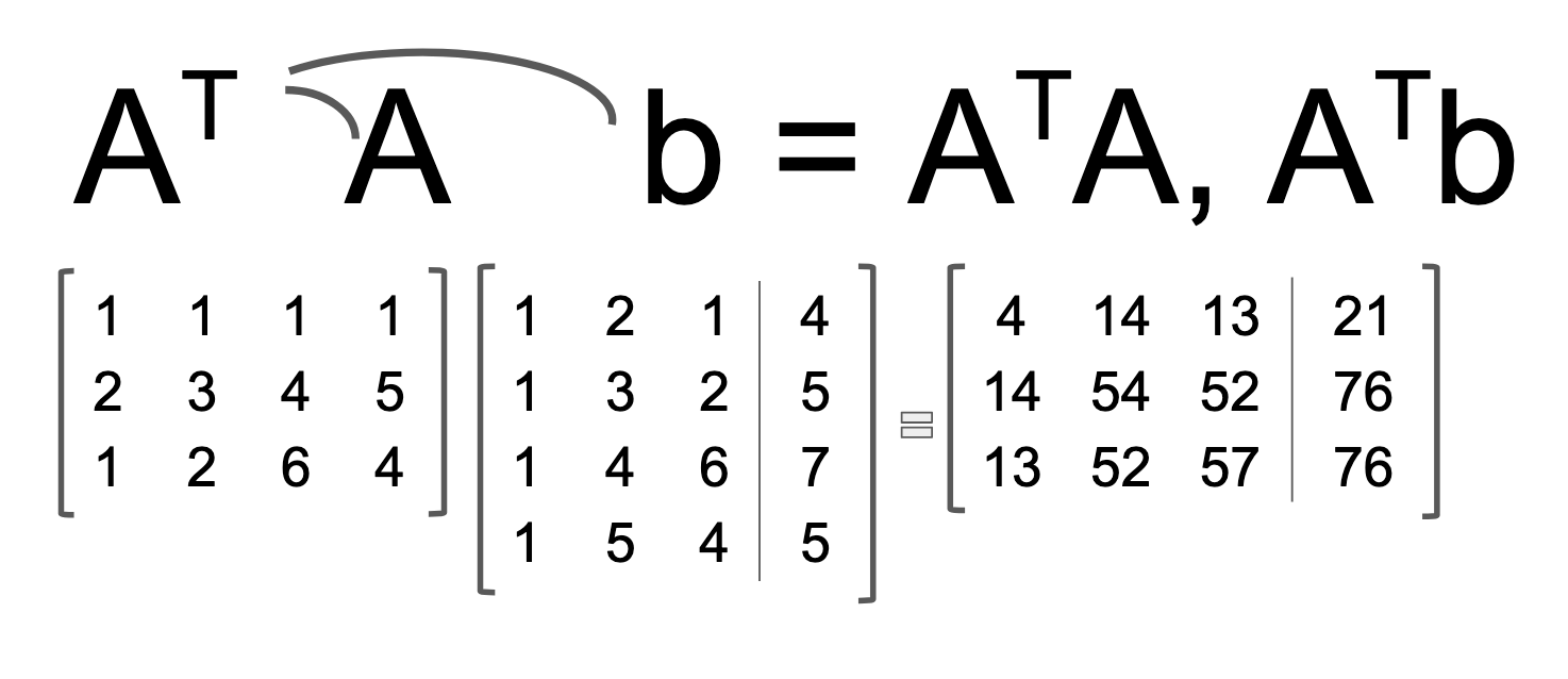
Now, this is crucial: The y-intercept is just a static number, so the value for its X0 is always 1. Thus Matrix A is defined:
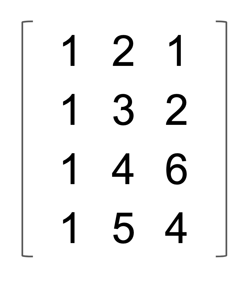
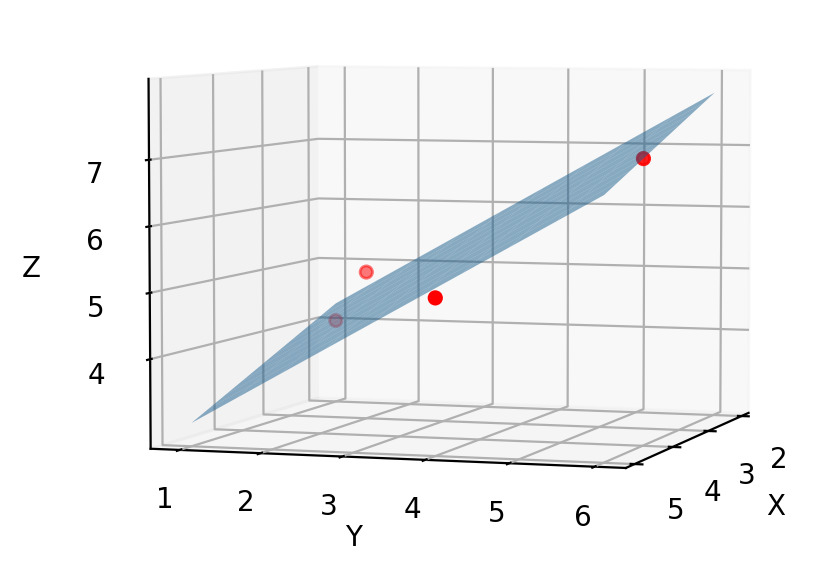
Let's pause and notice something about Matrix A. First thing: Matrix A is rectangular. It's not exactly a spreadsheet with 10,000 rows, but it's still a tall rectangular matrix. If we had one data point fewer, all three points would lie on a plane, since a plane can be defined by three points (linearly independent, of course). What transforms Matrix A into a problem requiring a least squares solution is the fourth point, which throws us off of the would-be plane.
Now that we have Matrix A, we can plug it into the formula ATAx̂=ATb. First we transpose A. Given Matrix A above, below is the equation we need to solve. From left to right, we have A transpose, multiplied by A, the coefficient vector x̂. On the right side of the equation, we see A transpose again, multiplying b, which is our given vector of "solutions," i.e. data points.
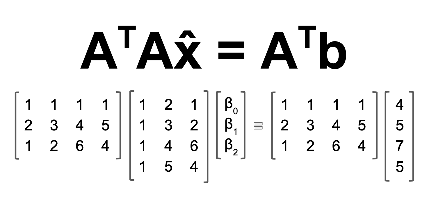
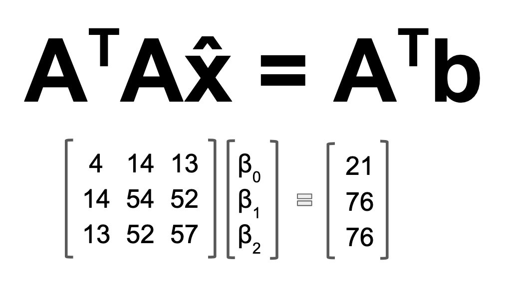
Now we are ready to rock and roll. First, we augment matrix A with vector b, and perform the matrix multiplication of ATA and ATb in one fell swoop, as it were. From our transformed solution vector, we are going to mine and extract the coefficient vector x̂: [β0,β1,β2]. Below is the completed matrix multiplication, with ATA and ATb shown on the right.
Remember this guy, from the Calculus example above?
- 4β0 + 14β1 + 13β2 = 21
- 14β0 + 54β1 + 52β2 = 76
- 13β0 + 52β1 + 57β2 = 76
Look familiar? Maybe I can show it thus:
- 4β0 + 14β1 + 13β2 = 21
- 14β0 + 54β1 + 52β2 = 76
- 13β0 + 52β1 + 57β2 = 76
It's the normal equations! The ones we have yet to solve... The totals we generated using the sum of squares summations. The numbers look eerily similar to the augmented matrix ATA|b. And there's a reason for that. Because, what we did in the Calculus example was compute the squared residuals, which is exactly what we do with the linear algebra formula. This is just ||ax-b||2. It looks the same because it is the same. (Later on, I will derive the linear algebra formula from ||ax-b||2).
The big win here is that it took us a lot of sloppy number crunching and summation module organization to get to this point in the Calculus. In Linear Algebra, you get to Step 50 in Step 2 (of course I'm exaggerating). From here, we can solve the equation just like we would solve any old Ax=b equation. Row reduce the augmented matrix, or decompose into LU, and find vector x.
I won't lie. There is still a lot of computation that goes into solving this system of equations. However, in the Calculus method, there are a whole bunch of steps, shown earlier in this post, to so much as arrive at a system of equations worth solving. The Linear Algebra formula is not only visually cleaner and easier to remember. It's also faster. It skips the whole aspect of computing partial derivatives.
Below are the computations, which I did by hand, to solve the system of equations. Initially I asked ChatGPT to double-check my work, but it failed miserably. So I used the Scipy function lstsq to double-check my work. I also did an LU decomposition with paper and pen just for sh*ts and giggles. Don't believe me? Here's the photographic evidence:
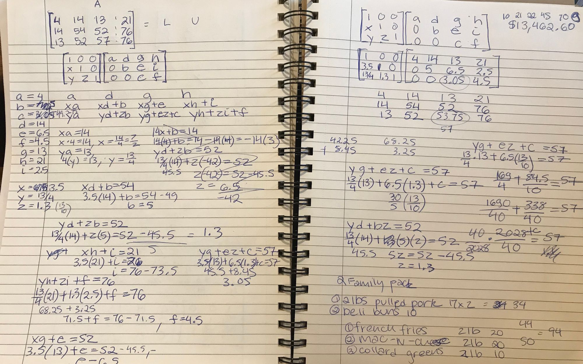
I prefer row reduction to LU decomposition, personally. Especially when I can do the row reduction methodically, and in a digital format, where I can copy and paste matrices, to easily move through steps. I like to record all of my transformations in a matrix E, on the lefthand side of the matrix being transformed. It helps me keep track of what I am doing, and what I have already done. When I stumble upon a computational error, it's easier to backtrack and figure out where I went wrong. As I move through further transformations, I change the previous transformations from black to grey, to indicate which transformations happened when.
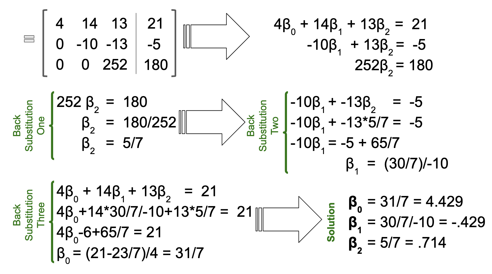
Matrix E is the lower triangular matrix on the left side, shown below. You can see that solving this equation involved three row transformations, each involving two rows. The first transformation was -3*Row One added to Row Two. The second, -3*Row One added to Row Three. The final transformation is -2 1/2*Row Two added to Row Three. The resulting upper triangular matrix, augmented with ATb, presents us with the new system of equations, which easily yields the solution vector, through back substitution (which I show in the following image).
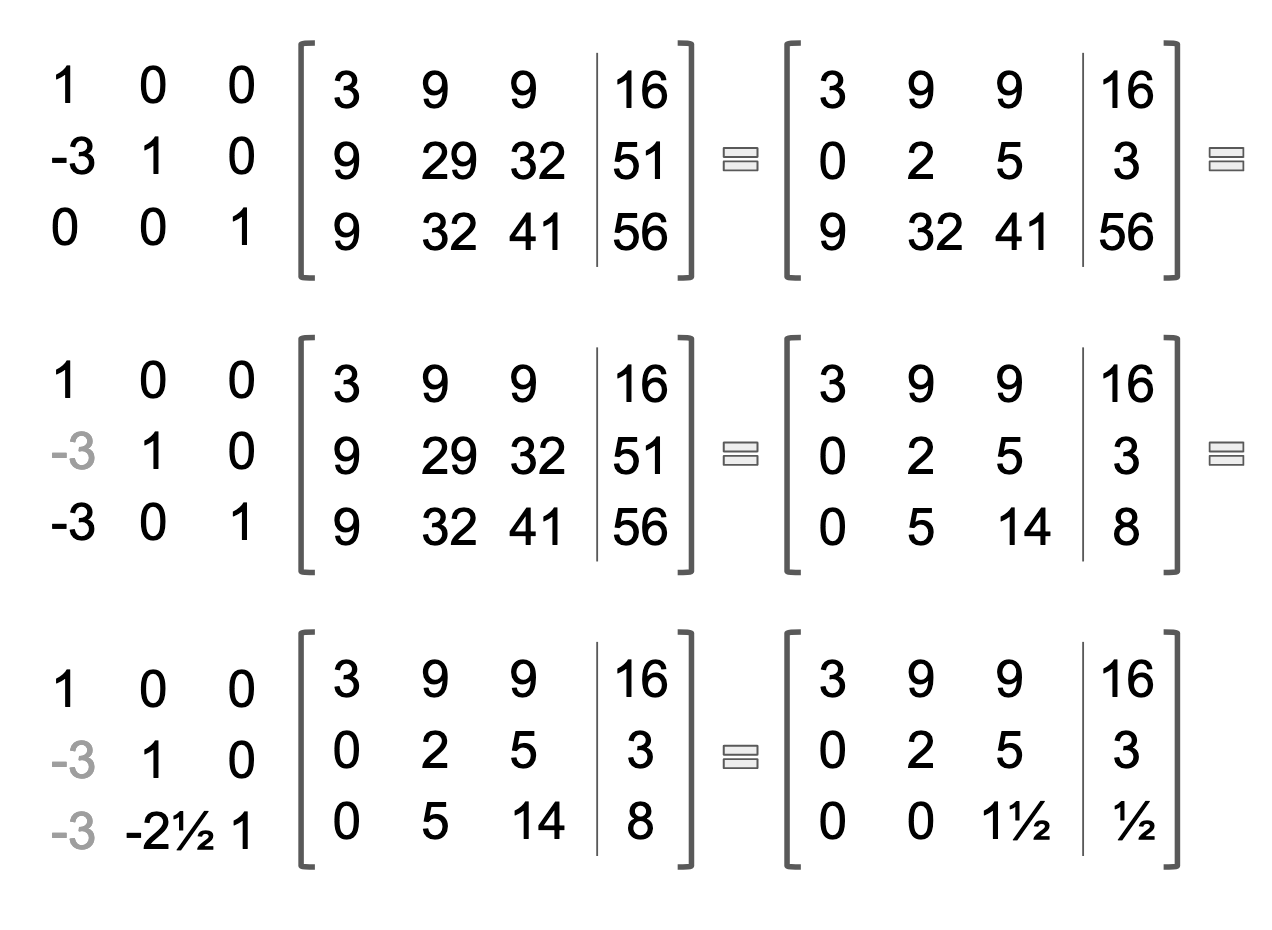
The computations involved in row reduction are not difficult: Just multiplying and adding! But with each step being cumulative, any mistake made early on can be difficult to unwind. Whenever I row reduce matrices, I am reminded of rebuilding the fallen domino structures, which my son used to make, when he went through his domino phase. One error will cause a cascade of errors, and may require the entire computation to be redone.
So what makes the linear algebra formula so fantastic, if it's still a treacherous slog at the end of the day? Well, a few things. First of all, just the appearance of the formula. The visual simplicity it provides gives a clear roadmap of what the formula is doing, i.e. finding x̂. In turn, this clarity of purpose commits itself to memory quite easily. The Calculus formula, on the other hand, has weak associations with x̂, which does not so much as appear in the formula. There is no indication that a vector of solutions is sought, and it's difficult to parse which symbols represent variables, versus which symbols represent known values.
The Calculus formula gets us to the same place, but without being clear about its goals or operations.
Not only do we skip the cumbersome steps of taking partial derivatives, but computationally it's more efficient besides. ATA and ATb can be generated simultaneously, although often instructions point you to do ATA and ATb separately. This way you can do away with the step of finding partial derivatives, entirely.
Derivation of Linear Algebra Least Squares Formula
How? The linear algebra version of the normal equations is derived from matrix subspace properties, like orthogonality of subspaces and orthogonal projection. Built-in properties of matrix multiplication, like summation and row reduction, do much of the computational work, which would ultimately be required, in the calculus formulas. For instance, we don't need to isolate each variable, taking one partial derivative at a time, because the process of row reduction isolates variables for us.
What follows is the derivation of ATAx=ATB from orthogonal projection:
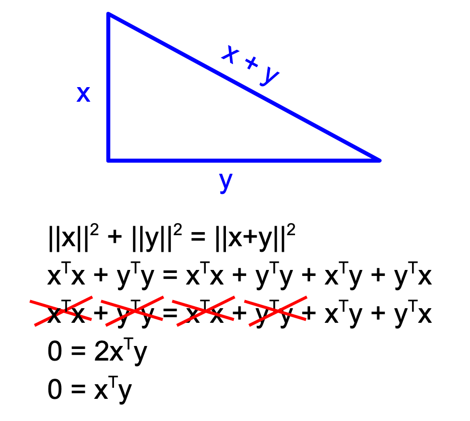
I. Figure A: When two vectors are orthogonal, their dot-product is zero (derivation from Pythagorean Theorem).
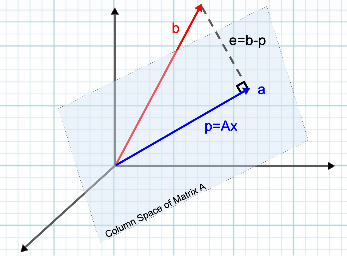
II. Figure B: Orthogonal Projection of any vector b onto line a "minimizes" error e, which gives us the formula aT(b-xa) = 0. This formula represents the dot product of vectors known to be orthogonal. (Line a is orthogonal to e, e=b-p, and p=xa).
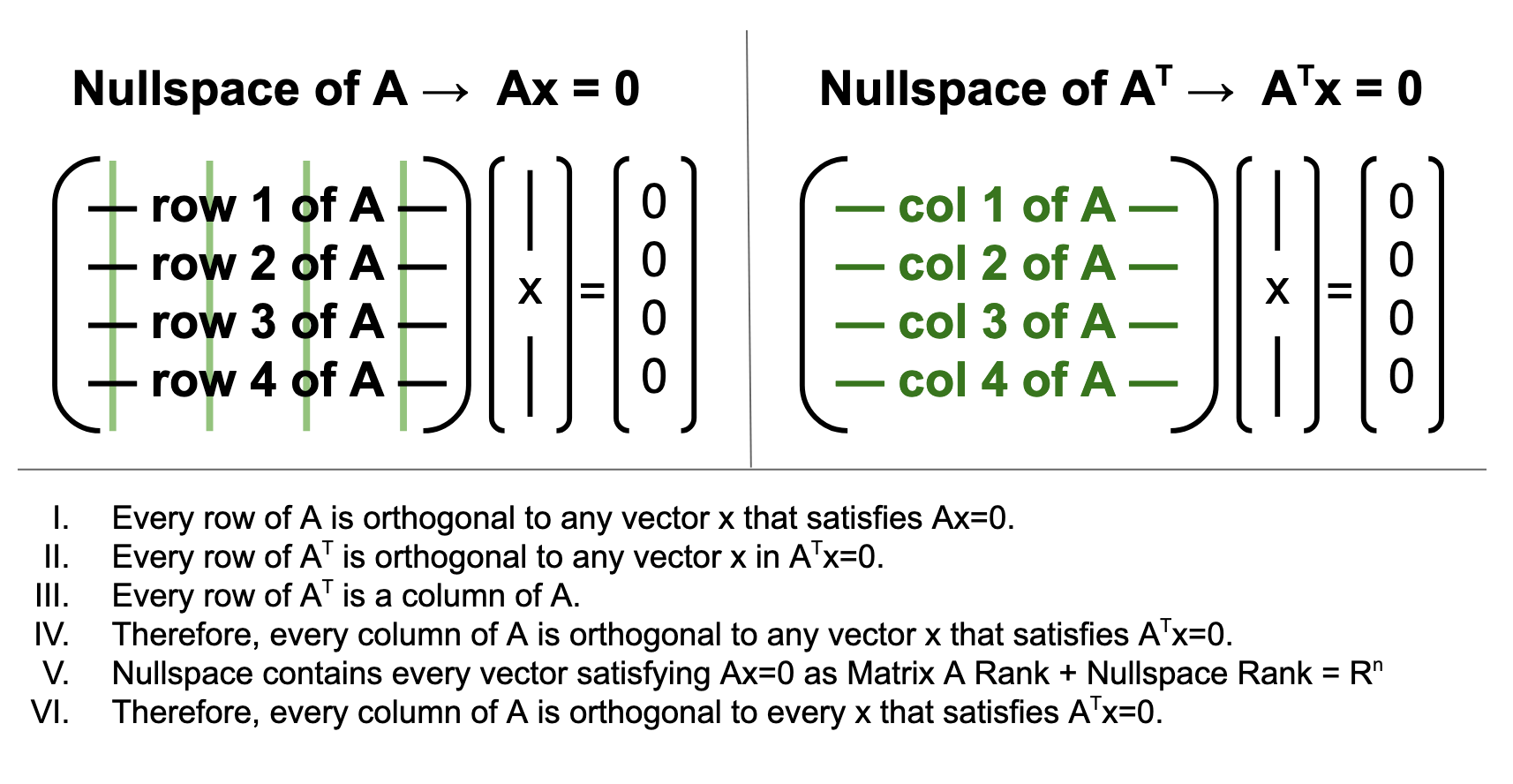
III. Figure C: All columns of A are orthogonal to all vectors in the nullspace of AT
IV. The Projection Matrix has the same properties as projection in one dimension
*Assumes errors are normally distributed
When you take the first derivative of a squared function, the result is linear. Thus, for squared functions, Linear Algebra really is the best option, because the underlying ("normal equations") will all be linear. Instead of minimizing the distance from your data to your model using calculus, you make an orthogonal projection. We need to find the intercept and the slope or weight of any additional variable, and if we organize the equations that need to be solved into a matrix, we can get the best solution via a few basic principles.
I. Column Space of Matrix A
Nullspace contains ALL vectors perpendicular to the nullspace (dimensions of each space add up to the full rank Rn). Thus
In Linear Algebra, two lines are orthogonal if they only meet at one point, zero. Why zero? Surely you can picture two lines crossing at a right angle sitting anywhere on the xy plane, right? Yes, but vectors always emerge from the origin. So you have to get used to thinking about vectors in space. Two planes are orthogonal if they only meet at the zero vector. That means they don't touch anywhere else. Thus A*B=0 The null space of a matrix. The dot product of two orthogonal vectors = 0.
In a loss function, the idea is to choose the function (doesn't have to be a line) that best fits the data. This means it gets as close as possible to every point in the data. As a theoretical concept this is simple. But how to actually achieve it with math is a little more complicated. It quickly dawns on you that the task involves solving a bunch of equations, simultaneously. In other words, you have to take the sum of every distance of Y from your line.
Different Loss Functions:
The abyss of finitude, and the promise of compute power
Polynomial, clumpy
Probabilistic loss function? Maximize the probability of a hypothesis, minimize the log likelihood.
Sometimes ATA produces a system that does not have a solution (linearly dependent cols, experiment replication). In this case, SVD-derived pseudo inverse can be used.