APIs vs. Tabulated Data
I wrote this post to help beginners at Python in extracting data from a CSV or Excel file, and flowing that data into a data frame in Pandas. This post is not about manipulating any kind of substantive data. This post is just about reading in a file, and getting your indexes set up properly.
If you are automating data flows in a professional environment, you want to pipe directly into an API. By connecting directly to an API, you eliminate these steps: Making a human (1) navigate to a data source, (2) download the applicable data tables, and (3) call the right file path in Pandas (or whatever other data frame interface tool you are using). These steps take only a few minutes, once you are familiar with the location of your desired data, but these locations can change. Also, in a large enterprise, where thousands or tens of thousands of data sets are used regularly, an entire team of (sad) people would be required to do these steps.
That said, there are many occasions where a data project pertains to an ad hoc study or a one-off question, and in these cases, connecting to an API is overkill. Also, many APIs lack historical data beyond a few years, in which case, tabulated data is the only option for obtaining historical numbers. In the worst cases, historical data will only be available in scans of paper data, which requires text recognition software, and wrangling for delimiters! But let's shun the thought of paper data, and continue on our quest of tidying basic tabulated data.
Read in CSV or XLS
First thing's first: import pandas as pd. OK, good. Now you are ready to work in Pandas! Below is an example of a Pandas read-in of an XLSX file. The same formula is available for CSV files. After importing Pandas into my Jupyter notebook, I used the following command:
df = pd.read_excel('filepath.extension'), followed by df.head() to take a look at what came through.
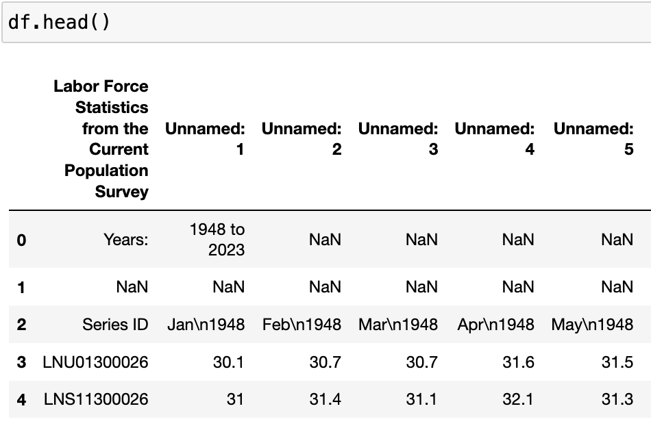
You can see that my data is from the Bureau of Labor Statistics, and contains some documentation in the header, indicating the source, the "Current Population Survey" and the years "1948-2023." Pandas did the best it could with the table, but ultimately it created a useless index in the top row, and gave us two full rows of empty cells ("NaN" means "Not a Number").
Clearly, the first three rows are totally useless to us. We know the data source, and we know the years in question. Thus, we can use the skiprows parameter in the pd.read_csv( ) function to skip those rows altogether. Since I will be using more than one data frame in my Jupyter notebook, I decided to give my data frame a better name than just df. I chose df_lfp (short for labor force participation). And I read in the file again, this time skipping the three useless rows:
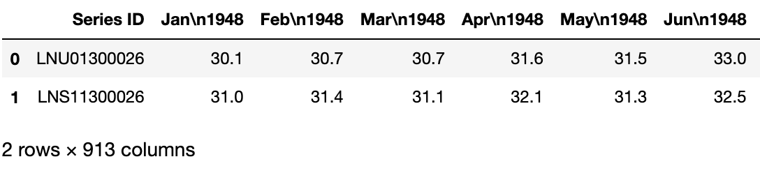
df_lfp = pd.read_excel('filepath.extension', skiprows=3)
We still have a bunch of problems that we need to fix, but this is looks much better already:
BLS Labor Force Participation data conveniently comes in two flavors: Raw and seasonally adjusted. Labor force participation has regular patterns of ebbs and flows, with seasonal workers entering and exiting the labor market in regular intervals. For the sake of data analysis, when looking at time series data, we must be very careful about seasonality. It would be embarrassing to predict, for example, that product sales are increasing at an increasing rate, (and to communicate the great news to upper management), only to discover that sales always increase during this season every year, and then dip right back down again.
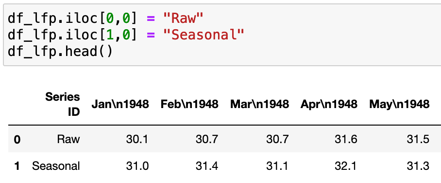
In this case, the BLS is sophisticated enough to seasonally adjust the data! Which is great. I wanted to keep both data series, because I am curious to see how they differ, once it comes time to chart them. However, I didn't want to lose track of which series was which, so I went ahead and changed the BLS codes "LNU0130026" and "LNS11300026" to Raw and Seasonal, respectively. I used the index locator function in Pandas to tell the code which cell values to change. The first number in brackets represents the row index, and the second, the column index, with the first column or row being zero.
You may be wondering, how do I change the first column, or the first row?!? You may have googled this repeatedly, and found only confusing answers. If that is the case, skip to the final section of this post.
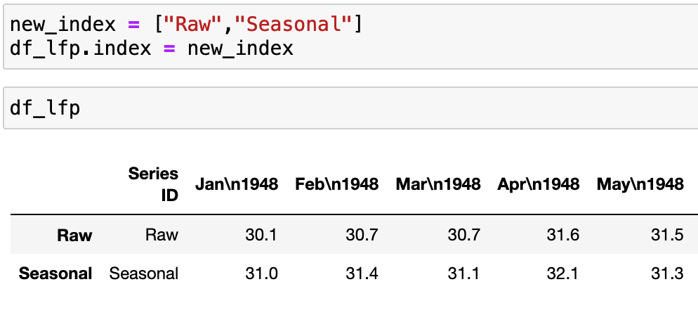
I went ahead and converted the "Raw" and "Seasonal" labels into a proper index.
Once I was satisfied that the new index was complete, and matched up properly to my data–in other words, that I hadn't swapped them or reversed the order by accident–I went ahead and dropped the first column of my data, which was called "Series ID" using axis=1 for columns (vertical axis). I typically use inplace=True when I know I am making a simple change that I do not wish to reverse, for which I cannot foresee any serious downstream consequences:
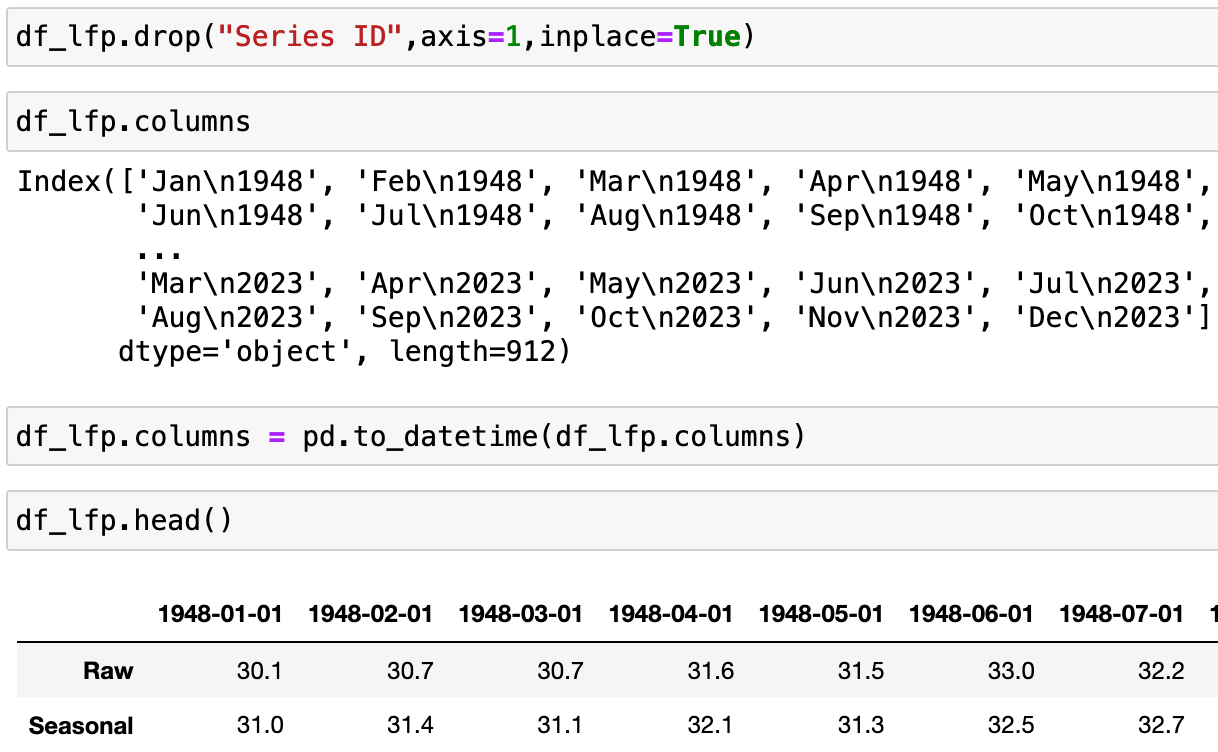
Finally, I passed my column labels into Pandas' to_datetime function, and it did a great job at converting my alphanumeric dates into a date index!
Index vs. Columns
I grew up doing data analysis in a Microsoft Excel environment. I find that growing up in a Microsoft Excel environment, there are a few simple translations of terms, which helped my transition into a Pandas environment.
1) First of all, your index column is not a column. Excel has a built-in index, in a way, which is the row numbers. In Excel, each row has a number, and these numbers do not themselves take up any space in the "spreadsheet." The numbers are tucked away in the margin. Normally, you add your own index labels, if desired. Thus, when it comes to navigating Pandas, it can feel like you should be able to delete that first column, if you want. But you can't! You can't delete the index any more than you can delete the row numbers in Excel. The index is a built-in hardwired feature of your data table, and it has to be there. The best you can do is rename the index, with new labels, a list, or a list comprehension.
2) Secondly, your column headings are not a row. Similar to point #1, Pandas "columns" are not your first row. In Excel, you are probably accustomed to having your column labels reside in the first row, which you then freeze for ease of use. You may not realize that you have, in fact, created a column index. Nor are your column headings called a "row index." You may be tempted to think of them as such, but they are not a row at all. If you want to know what your horizontal index labels are, use the method df.columns. This will give you the name of your columns. If you want to know your index labels, use df.index.
3) Finally, neither your columns nor index are mutable. In other words, you cannot change the values in the cells through reassignment, as you normally might. The only way to change the values of these cells is to pass a dictionary, which changes the data at the array level, rather than the data frame level.
Just remember your first column is your index labels. And your first row is your column labels. Your index and column labels are not truly rows or columns. You can't delete them. You can only rename them!